Weighted Least Squares
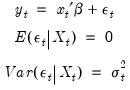
Suppose that you have heteroskedasticity of known form, where the conditional error variances are given by

. The presence of heteroskedasticity does not alter the bias or consistency properties of ordinary least squares estimates, but OLS is no longer efficient and conventional estimates of the coefficient standard errors are not valid.
If the variances

are known up to a positive scale factor, you may use weighted least squares (WLS) to obtain efficient estimates that support valid inference. Specifically, if
 | (21.22) |
and we observe

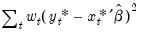
, the WLS estimator for

minimizes the weighted sum-of-squared residuals:
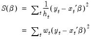 | (21.23) |
with respect to the

-dimensional vector of parameters

, where the weights

are proportional to the inverse conditional variances. Equivalently, you may estimate the regression of the square-root weighted transformed data
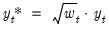
on the transformed
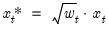
.
In matrix notation, let

be a diagonal matrix containing the scaled

along the diagonal and zeroes elsewhere, and let

and

be the matrices associated with

and

. The WLS estimator may be written,
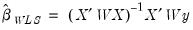 | (21.24) |
and the default estimated coefficient covariance matrix is:
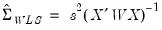 | (21.25) |
where
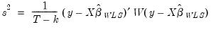 | (21.26) |
is a d.f. corrected estimator of the weighted residual variance.
To perform WLS in EViews, open the equation estimation dialog and select a method that supports WLS such as then click on the tab. (You should note that weighted estimation is not offered in equations containing ARMA specifications, nor is it available for some equation methods, such as those estimated with ARCH, binary, count, censored and truncated, or ordered discrete choice techniques.)
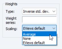
You will use the three parts of the section of the tab to specify your weights.
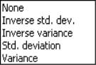
The dropdown is used to specify the form in which the weight data are provided. If, for example, your weight series VARWGT contains values proportional to the conditional variance, you should select . Alternately, if your series INVARWGT contains the values proportional to the inverse of the standard deviation of the residuals you should choose
Next, you should enter an expression for your weight series in the edit field.
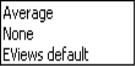
Lastly, you should choose a scaling method for the weights. There are three choices: , , and (in some cases) . If you select , EViews will, prior to use, scale the weights so that the

sum to

. The specification scales the weights so the square roots of the

sum to

. (The latter square root scaling, which offers backward compatibility to EViews 6 and earlier, was originally introduced in an effort to make the weighted residuals
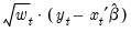
comparable to the unweighted residuals.) Note that the EViews default method is only available if you select as weighting .
Unless there is good reason to do so, we recommend that you employ with scaling, even if it means you must transform your weight series. The other weight types and scaling methods were introduced in EViews 7, so equations estimated using the alternate settings may not be read by prior versions of EViews.
We emphasize the fact that

and

are almost always invariant to the scaling of weights. One important exception to this invariance occurs in the special case where some of the weight series values are non-positive since observations with non-positive weights will be excluded from the analysis unless you have selected scaling, in which case only observations with zero weights are excluded.
As an illustration, we consider a simple example taken from Gujarati (2003, Example 11.7, p. 416) which examines the relationship between compensation (Y) and index for employment size (X) for nine nondurable manufacturing industries. The data, which are in the workfile “Gujarati_wls.WF1”, also contain a series SIGMA believed to be proportional to the standard deviation of each error.
To estimate WLS for this specification, open an equation dialog and enter
y c x
as the equation specification.
Click on the tab, and fill out the section as depicted here. We select as our , and specify “1/SIGMA” for our . Lastly, we select as our method.
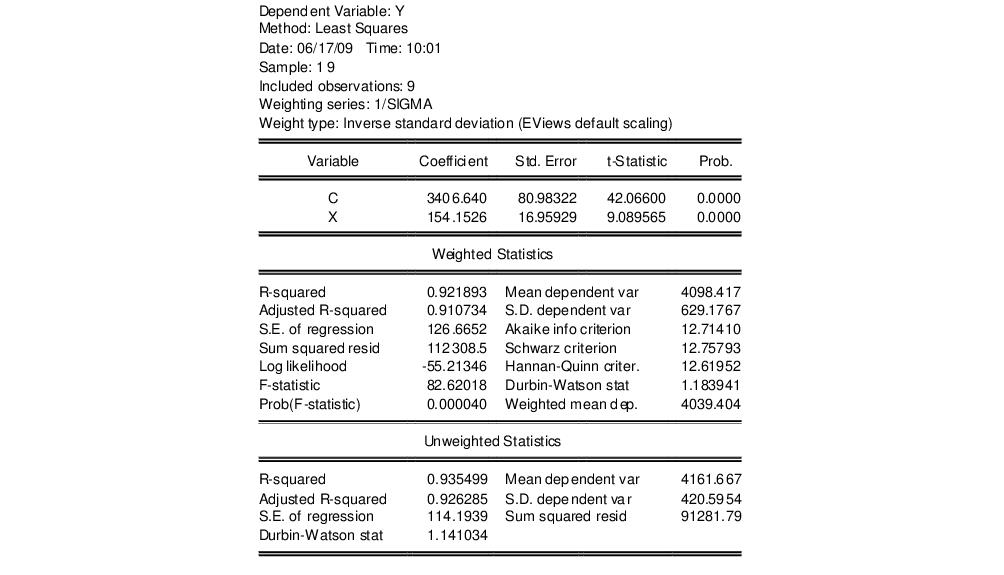
Click on to estimate the specified equation. The results are given by:
The top portion of the output displays the estimation settings which show both the specified weighting series and the type of weighting employed in estimation. The middle section shows the estimated coefficient values and corresponding standard errors, t-statistics and probabilities.
The bottom portion of the output displays two sets of statistics. The show statistics corresponding to the actual estimated equation. For purposes of discussion, there are two types of summary statistics: those that are (generally) invariant to the scaling of the weights, and those that vary with the weight scale.
The “R-squared”, “Adjusted R-squared”, “F-statistic” and “Prob(F-stat)”, and the “Durbin-Watson stat”, are all invariant to your choice of scale. Notice that these are all fit measures or test statistics which involve ratios of terms that remove the scaling.
One additional invariant statistic of note is the “Weighted mean dep.” which is the weighted mean of the dependent variable, computed as:
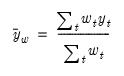 | (21.27) |
The weighted mean is the value of the estimated intercept in the restricted model, and is used in forming the reported F-test.
The remaining statistics such as the “Mean dependent var.”, “Sum squared resid”, and the “Log likelihood” all depend on the choice of scale. They may be thought of as the statistics computed using the weighted data,

and

. For example, the mean of the dependent variable is computed as
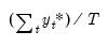
, and the sum-of-squared residuals is given by
. These values should not be compared across equations estimated using different weight scaling.
Lastly, EViews reports a set of . As the name suggests, these are statistics computed using the unweighted data and the WLS coefficients.