An Example
Greene (2008, page 685) uses an ARDL model on data from a number of quarterly US macroeconomic variables between 1950 and 2000. In particular, he estimates an ARDL model using the log of real consumption as the dependent variable, and the log of real GDP as a single regressor (along with a constant).
We can open the Greene data with the following EViews command:
wfopen http://www.stern.nyu.edu/~wgreene/Text/Edition7/TableF5-2.txt
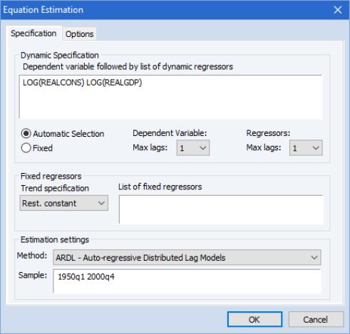
Next we bring up the ARDL estimation dialog by clicking on and using the Method combo to change the estimation method to ARDL.
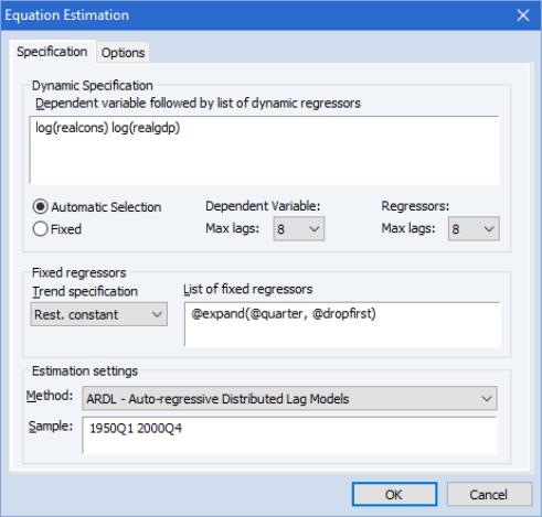
Following Greene's example, we estimate an ARDL model with the log of real consumption as the dependent variable, and log GDP as the regressor, by entering:
log(realcons) log(realgdp)
in the Dynamic Specification area. We choose to perform Automatic Selection, with a maximum of 8 lags (two years) for both the dependent variable and dynamic regressors.
Greene includes a full set of quarterly dummies as fixed regressors, which we can include by choosing Constant (Level) as the trend specification, and then adding the expression “@expand(@quarter, @droplast)” in the Fixed regressors box.
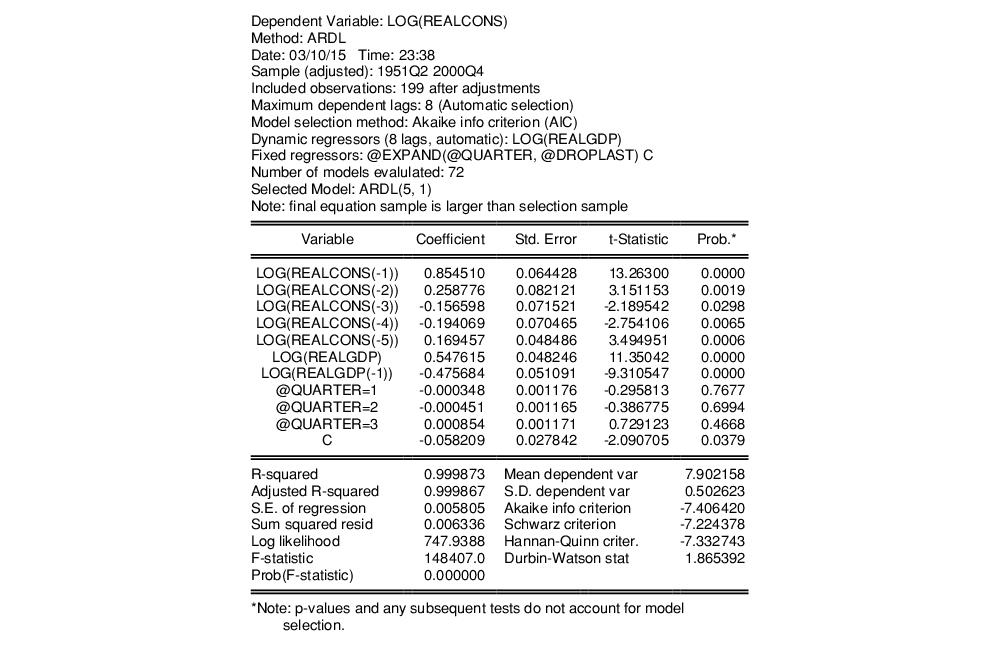
We do not make any changes to the Options tab, leaving all settings at their default value. The results are shown below:
The first part of the output gives a summary of the settings used during estimation. Here we see that automatic selection (using the Akaike Information Criterion) was used with a maximum of 8 lags of both the dependent variable and the regressor. Out of the 72 models evaluated, the procedure has selected an ARDL(5,1) model - 5 lags of the dependent variable, LOG(REALCONS), and a single lag (along with the level value) of LOG(REALGDP).
EViews also notes that since the selected model has fewer lags than the maximum, the sample used in the final estimation will not match that used during selection.
The rest of the output is standard least squares output for the selected model. Note that each of the regressors (with the exception of the quarterly dummies) is significant, and that the coefficient on the one period lag of the dependent variable, LOG(REALCONS), is quite high, at 0.85.
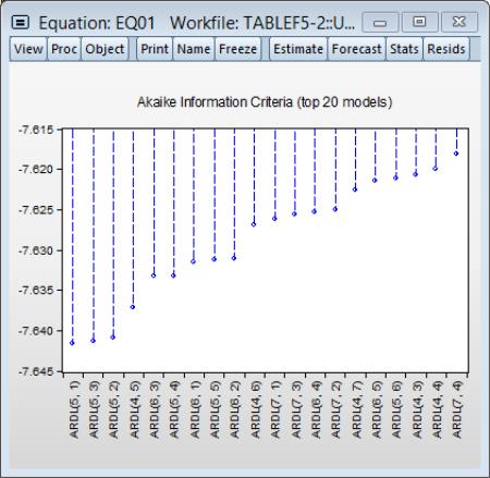
To view the relative superiority of the selected model against alternatives, we click on V to view a graph of the AIC of the top twenty models.
The selected ARDL(5,1) model was only slightly better than an ARDL(5,2) model, which was in turn only slightly better than an ARDL(5,3). It is notable that the top three models all use five lags of the dependent variable.
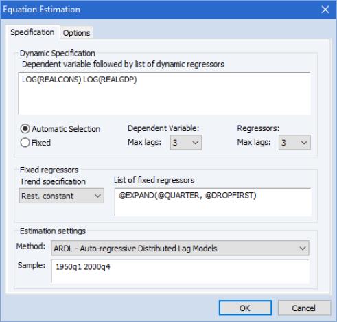
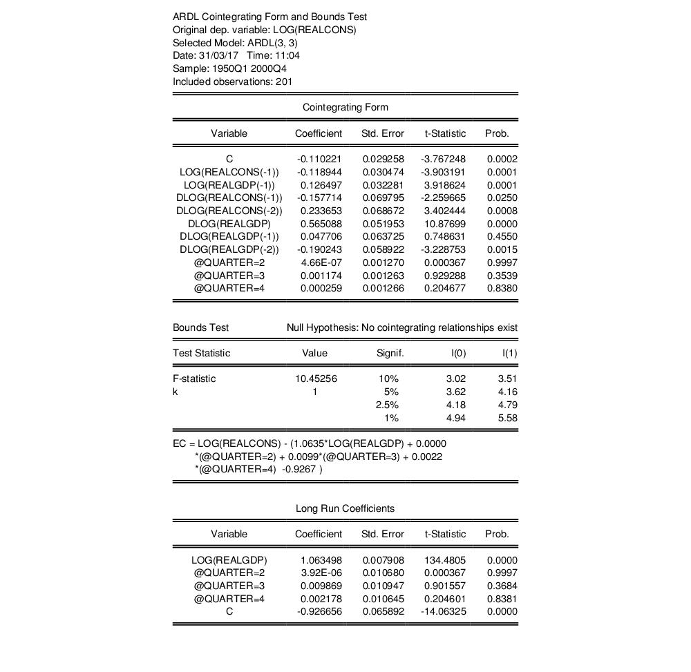
Rather than using automatic selection to choose the best model, Greene (Example 20.4) analyzes these data with a fixed ARDL(3,3) model. We can replicate this by pressing the button to bring up the Equation Estimation dialog again. We change the number of lags on both dependent and regressors to 3, and then select the Fixed radio button to switch off automatic selection.
The results of this estimation are:
The one-period lag on the dependent variable remains high, at 0.72, and again all coefficients are significant (with the exception of the dummies).
We can then examine the long-run coefficients by selecting .
The long-run coefficients, at the bottom of the output, show that the long-run impact of a change in log(REALGDP) on log(REALCONS) has essentially no lagged-effects. The long-run change is very close to being equal to the initial change (the coefficient is close to one).
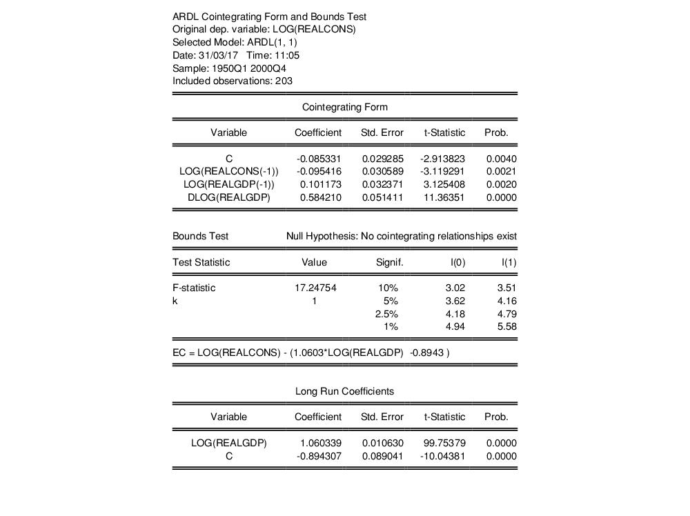
In a second example, Example 20.5, Greene examines an ARDL(1,1) model's cointegrating form. To perform this in EViews, we again bring up the dialog and change the number of lags to 1 for both dependent and regressors, remove the quarterly dummies, and then click OK.
Following estimation, we click on to bring up the cointegrating relationship view: