Example
We consider here an example of Lasso estimation using the prostate cancer data described in multiple sources such as the textbook by Hastie, Tibshirani, and Friedman (2017, 3.4, p. 61). The regressors are log(cancer volume) (LCAVOL), log(prostate weight) (LWEIGHT), age, the logarithm of the amount of benign prostatic hyperplasia (LBPH), seminal vesicle invasion (SVI), log(capsular penetration) (LCP), Gleason score (GLEASON) and percentage Gleason score 4 or 5 (PGG45). The dependent variable is the logarithm of prostate-specific antigen (LPSA). The “prostate.wf1” workfile containing these data obtained from the authors’ website is available in your EViews example data.
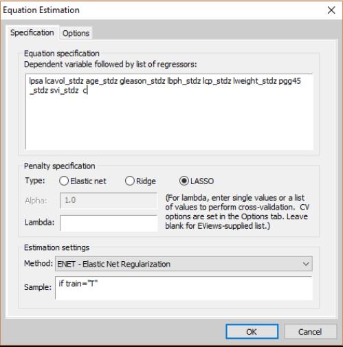
To estimate this model, open the elastic net dialog and fill it out as depicted:
In order to match the directions given in the accompanying file “prostate.info.txt,” also from the authors’ website, we have already standardized the regressors across the length of the dataset. The lambda field is blank to allow EViews to calculate the lambda path and use cross-validation to find the model with the smallest error. We have also specified the sample to include only the training data. On the options page we choose 10-fold cross-validation as directed and leave the other values at their defaults. Click on to estimate this specification and display the results.
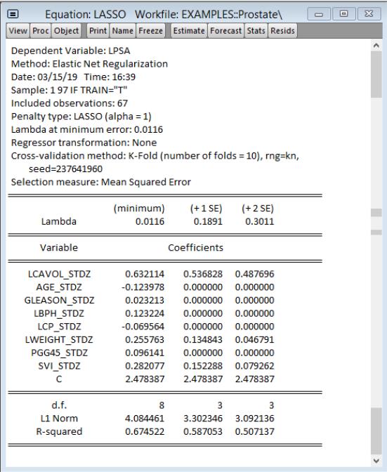
Comparison with Table 3.3 reported in Hastie, Tibshirani, and Friedman shows that while the coefficients in the +1SE column in the EViews output are very close, they are not an exact match. While there are a few potential sources for this difference, it is most likely due to randomness associated with the cross-validation procedure.
Next we will view the evolution of the coefficients with respect to the lambda penalty:
=
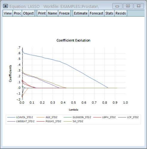
As expected, as the penalization increases, the complexity of the model decreases and the coefficients gradually shrink to zero. The model at +1SE (lambda = 0.189) chosen by cross-validation is after most of the coefficients have fallen out of the model.
By forecasting over the test data, EViews calculates a root mean squared error for the Lasso model of 0.632.
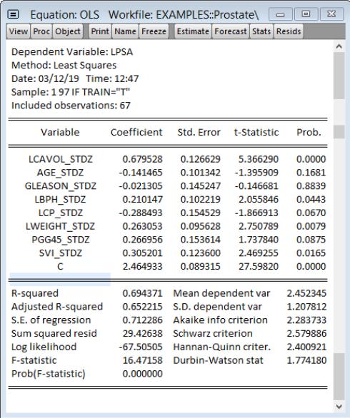
For comparison, we have also analyzed the same data with an OLS model:
After forecasting over the test data EViews finds a higher root mean squared error for the OLS model of 0.722, compared to 0.632 for the Lasso model. A similar calculation for the ridge model also leads to a lower root mean squared error (0.640) compared to least squares. The regularized regression models have superior forecast performance compared to the OLS model.