Estimating Functional Coefficients Models in EViews
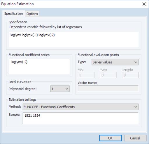
To estimate a functional coefficient model, from the main EViews menu and select from the main dropdown menu near the bottom of the dialog to display the functional coefficients dialog:
• In the edit field you should enter your dependent variable followed by a list of functional coefficient regressors. Here, LOGLYNX is the dependent variable, and the two lag variables LOGLYNX(-1) and LOGLYNX(-2) will have functional coefficients.
• In the variable edit field, you will enter the

variable upon which the functional coefficients depend. Here the coefficients will vary with LOGLYNX(-2).
• In the section, the dropdown allows you to choose the degree of the regression approximation. For example, local linear regression will set this to 1.
• The options group allows you to control the evaluation points for the estimation. The dropdown specifies the source of the evaluation points. By default, the values at which we evaluate the functional coefficients are set to the actual data

. If you wish to control the evaluation points, you may select and provide a minimum, maximum, and length, to create the corresponding evenly spaced grid. Alternatively, if the custom grid is stored as a vector in the workfile, selectand enter the name of the vector.
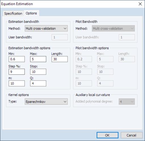
The tab allows you to specify settings associated with bandwidth selection methods and kernel types.
• From the group dropdown, you may select the method for choosing the estimation bandwidth. You may choose between: , , , (default), , , , and . If a bandwidth is requested, you will be prompted to enter a bandwidth.
• Associated with the automated bandwidth methods are bandwidth search options specifying the , , , , and settings. The first three set the minimum, maximum, and length of the bandwidth grid over which to search for an optimal bandwidth. The last two determine the increment by which to increase the grid value when searching, and how many consecutive failures to improve upon the optimal bandwidth are permitted before the search is terminated. Note here that the search also terminates whenever either the maximum is reached, or the number of bandwidths searched reaches the length specified. Furthermore, when the bandwidth mechanism is , the number of forecast steps is specified in the edit field, and the number of sub-series to evaluate may be specified under (see
“Pilot Bandwidth”).
• Next, the type of kernel used in estimation may be specified in the dropdown. You may choose between: , , (default), , , and . Note that the types are ordered from least to most smooth.
• Lastly, when the estimation bandwidth requires a pilot bandwidth, the latter may be specified group dropdown. The options here follow the same principles outlined for the main bandwidth selection method. Since a pilot bandwidth procedure also requires an auxiliary estimation degree, the latter can be specified from the group by selecting an appropriate value from the dropdown. Note here that this auxiliary degree is in addition to the main polynomial degree specified on the tab. In other words, if the main polynomial degree is 1, and the auxiliary polynomial degree is 2, then the pilot polynomial degree will be equal to 3.
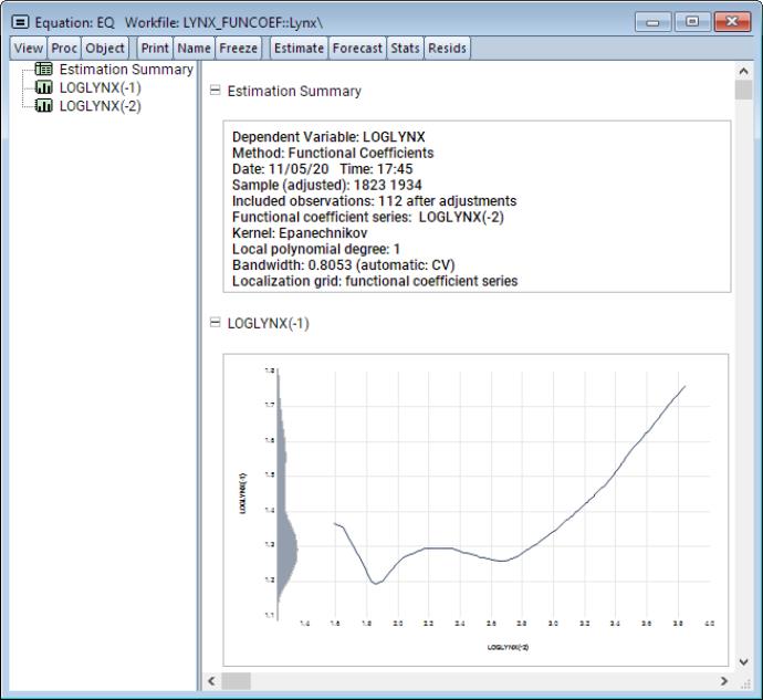
Once you have specified your functional coefficients regression specification and set the options, clicking on estimates the model and displays results in the form of spool output:
The shows the functional coefficients estimation settings. Below these settings are graphs showing the functional coefficients relationships for each of the regressors.


 variable upon which the functional coefficients depend. Here the coefficients will vary with LOGLYNX(-2).
 . If you wish to control the evaluation points, you may select Uniform grid and provide a minimum, maximum, and length, to create the corresponding evenly spaced grid. Alternatively, if the custom grid is stored as a vector in the workfile, select Vector values and enter the name of the vector.
