An Example
As an example of using Mixed Frequency VARs in EViews, we will perform similar analysis to that in Ghysels (2016). The analysis involves monthly industrial production, inflation and unemployment data for the US between 1949 and 2011, and quarterly US GDP data over the same period. The data are provided in the two-page workfile “Kansfed.WF1”.
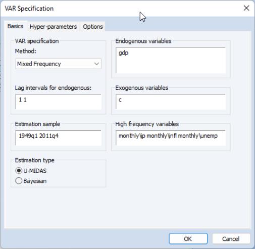
Following Ghysels, we will estimate a mixed frequency VAR model with a single lag. Ensuring we have the page selected, we click on menu item and fill in the details of our VAR. To begin we will estimate a U-MIDAS model with the single quarterly variable, GDP, and three monthly variables:
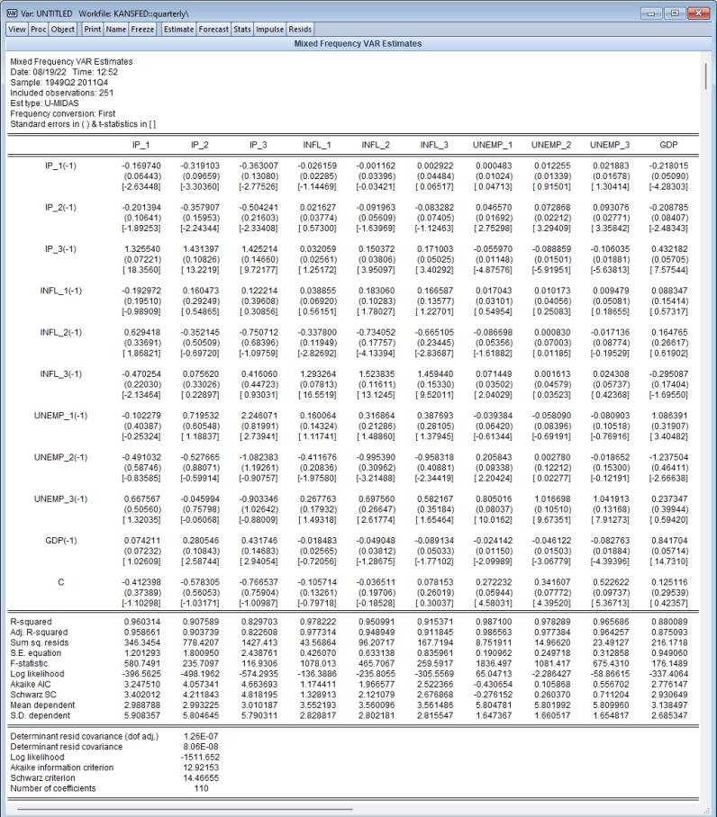
Clicking on produces the result:
Each of the monthly variables, IP, INFL and UNEMP have been transformed into three separate variables in the quarterly VAR, one variable for each month in the quarter. The “_i” suffix is used to distinguish each month.
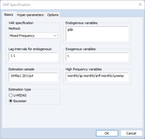
In his paper, rather than estimating with U-MIDAS, Ghysels estimates using a Bayesian prior, which we can replicate by clicking to bring up the dialog and selecting as the :
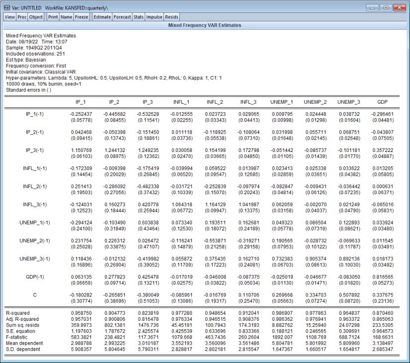
Clicking on produces:
These results are in line with those reported in Table 5 of Ghysels and show a reasonable difference from the U-MIDAS/classical VAR we first estimated – for example the coefficient on the first monthly observation of IP on a single quarterly lag of itself changes from -0.17 to -0.25.
