Examples
We demonstrate the use of the optimize command with several examples. To begin, we consider a regression problem using a workfile created with the following set of commands:
wfcreate u 100
rndseed 1
series e = nrnd
series x1 = 100*rnd
series x2 = 30*nrnd
series x3 = -4*rnd
group xs x1 x2 x3
series y = 3 + 2*x1 + 4*x2 + 5*x3 + e
equation eq1.ls y c x1 x2 x3
These commands create a workfile with 100 observations, and then generate some random data for series X1, X2 and X3, and E (where E is drawn from the standard normal distribution). The series Y is created as 3+2*X1+4*X2+5*X3 + E.
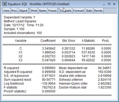
To establish a baseline set of results for comparison, we regress Y against a constant, X1, X2, and X3 using the built-in least squares method of the EViews equation object. The results view for the resulting equation EQ1 contains the regression output:
Next we use the optimize command with the least squares method to estimate the coefficients in the regression problem. Running a program with the following commands produces the same results as the built-in regression estimator:
subroutine leastsquares(series r, vector beta, series dep, group regs)
r = dep - beta(1) - beta(2)*regs(1) - beta(3)*regs(2) - beta(4)*regs(3)
endsub
series LSresid
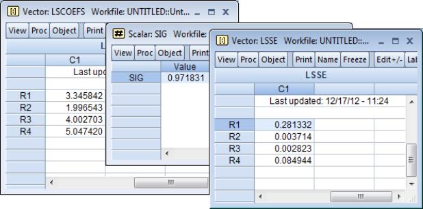
vector(4) LSCoefs
lscoefs = 1
optimize(ls=1, finalh=lshess) leastsquares(LSresid, lscoefs, y, xs)
scalar sig = @sqrt(@sumsq(LSresid)/(@obs(LSresid)-@rows(LSCoefs)))
vector LSSE = @sqrt(@getmaindiagonal(2*sig^2*@inverse(lshess)))
We begin by defining the LEASTSQUARES subroutine which computes the regression residual series R, using the parameters given by the vector BETA, the dependent variable given by the series DEP, and the regressors provided by the group REGS. All of these objects are arguments of the subroutine which are passed in when the subroutine is called.
Next, we declare the LSRESID series and a vector of coefficients, LSCOEFS, which we arbitrarily initialize at a value of 1 as starting values.
The optimize command is called with the “ls” option to indicate that we wish to perform a least squares optimization. The “finalh” option is included so that we save the estimated Hessian matrix in the workfile for use in computing standard errors of the estimates. optimize will find the values of LSCOEFS that minimize the sum of squared values of LSRESID as computed using the LEASTSQUARES subroutine.
Once optimization is complete, LSCOEFS contains the point estimates of the coefficients. For least squares regression, the standard error of the regression

is calculated as the square root of the sum of squares of the residuals, divided by

. We store

in the scalar SIG. Standard errors may be calculated from the Hessian as the square root of the diagonal of

. We store these values in the vector LSSE.
The coefficients in LSCOEFS, standard error of the regression

in SIG, and coefficient standard errors in LSSE, all match the results in EQ1.
Alternately, we may use optimize to estimate the maximum likelihood estimates of the regression model coefficients. Under standard assumptions, an observation-based contribution to the log-likelihood for a regression with normal error terms is of the form:
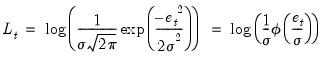 | (10.1) |
The following code obtains the maximum likelihood estimates for this model:
subroutine loglike(series logl, vector beta, series dep, group regs)
series r = dep - beta(1) - beta(2)*regs(1) - beta(3)*regs(2) - beta(4)*regs(3)
logl = @log((1/beta(5))*@dnorm(r/beta(5)))
endsub
series LL
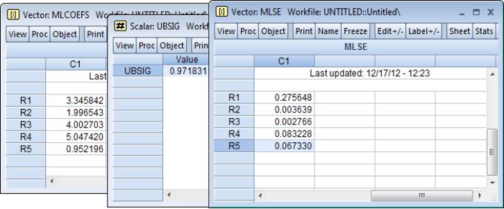
vector(5) MLCoefs
MLCoefs = 1
MLCoefs(5) = 100
optimize(ml=1, finalh=mlhess, hess=numeric) loglike(LL, MLCoefs, y, xs)
vector MLSE = @sqrt(@getmaindiagonal(-@inverse(mlhess)))
scalar ubsig = mlcoefs(5)*@sqrt(@obs(LL)/(@obs(LL) - @rows(MLCoefs) + 1))
%status = @optmessage
statusline {%status}
The subroutine LOGLIKE computes the regression residuals using the coefficients in the vector BETA, the dependent variable series given by DEP, and the regressors in the group REGS. Given R, the subroutine evaluates the individual log-likelihood contributions and puts the results in the argument series LOGL.
The next lines declare the series LL to hold the likelihood contributions and the coefficient vector BETA to hold the controls. Note that the coefficient vector, BETA, has five elements instead of the four used in least-squares optimization, since we are simultaneously estimating the four regression coefficients and the error standard deviation

. We arbitrarily initialize the regression coefficients to 1 and the distribution standard deviation to 100.
We set the maximizer to perform a maximum likelihood based estimation using the “ml=” option and to store the OPG Hessian in the workfile in the sym objected MLHESS. The coefficient standard errors for the maximum likelihood estimates may be calculated as the square root of the main diagonal of the negative of the inverse of MLHESS. We store the estimated standard errors in the vector MLSE.
Although the regression coefficient estimates match those in the baseline, the ML estimate of

in the fifth element of BETA differs. You may obtain the corresponding unbiased estimate of sigma by multiplying the ML estimate by multiplying BETA(5) by

, which we calculate and store in the scalar UBSIG.
Note also that we use @optmessage to obtain the status of estimation, whether convergence was achieved and if so, how many iterations were required. The status is reported on the statusline after the optimize estimation is completed.
The next example we provide shows the use of the “grads=” option. This example re-calculates the least-squares example above, but provides analytic gradients inside the subroutine. Note that for a linear least squares problem, the derivatives of the objective with respect to the coefficients are the regressors themselves (and a series of ones for the constant):
subroutine leastsquareswithgrads(series r, vector beta, group grads, series dep, group regs)
r = dep - beta(1) - beta(2)*regs(1) - beta(3)*regs(2) - beta(4)*regs(3)
grads(1) = 1
grads(2) = regs(1)
grads(3) = regs(2)
grads(4) = regs(3)
endsub
series LSresid
vector(4) LSCoefs
lscoefs = 1
series grads1
series grads2
series grads3
series grads4
group grads grads1 grads2 grads3 grads4
optimize(ls=1, grads=3) leastsquareswithgrads(LSresid, lscoefs, grads, y, xs)
Note that the series for the gradients, and the group containing those series, were declared prior to calling the optimize command, and that the subroutine fills in the values of the series inside the gradient group.
Up to this point, our examples have involved the evaluation of series expressions. The optimizer does, however, work with other EViews commands. We could, for example, compute the least squares estimates using the optimizer to “solve” the normal equation
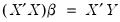
for

. While the optimizer is not a solver, we can trick it into solving that equation by creating a vector of residuals equal to
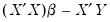
, and asking the optimizer to find the values of

that minimize the square of those residuals:
subroutine local matrixsolve(vector rvec, vector beta, series dep, group regs)
stom(regs, xmat)
xmat = @hcat(@ones(100), xmat)
stom(dep, yvec)
rvec = @transpose(xmat)*xmat*beta - @transpose(xmat)*yvec
rvec = @epow(rvec,2)
endsub
vector(4) MSCoefs
MSCoefs = 1
vector(4) rvec
optimize(min=1) matrixsolve(rvec, mscoefs, y, xs)
Since we will be using matrix manipulation for the objective function, the first few lines of the subroutine convert the input dependent variable series and regressor group into matrices. Note that the regressor group does not contain a constant term upon input, so we append a column of ones to the regression matrix XMAT, using the @hcat command.
Lastly, we use the optimize command to find the minimum of a simply function of a single variable. We define a subroutine containing the quadratic form, and use the optimize command to find the value that minimizes the function:
subroutine f(scalar !y, scalar !x)
!y = 5*!x^2 - 3*!x - 2
endsub
create u 1
scalar in = 0
scalar out = 0
optimize(min) f(out, in)
This example first creates an empty workfile and declares two scalar objects, IN and OUT, for use by the optimizer. IN will be used as the parameter for optimization, and is given an arbitrary starting value of 0. The subroutine F calculates the simple quadratic formula:
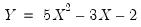 | (10.2) |
After running this program the value of IN will be 0.3, and the final value of OUT (evaluated at the optimal IN value) is -2.45. As a check we can manually calculate the minimal value of the function by taking derivatives with respect to X, setting equal to zero, and solving for X:
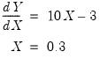 | (10.3) |