Examples
To illustrate the estimation of panel cointegration models in EViews, we follow Kao, Chiang, and Chen (KCC, 1999) who apply panel cointegration analysis to the study of economic growth by estimating the cointegrating relationship for total factor productivity and domestic and foreign R&D capital stock.
The KCC data, which we provide in the workfile “tfpcoint.WF1” consist of annual data on log total factor productivity (LTFP), log domestic (LRD), and log foreign (LFRD) R&D capital stock for 22 countries for the years 1971 to 1990. We consider estimation of simple pooled FMOLS and DOLS estimators for the cointegrating vectors as in Table 4(i) (p. 703) and Table 5(i) (p. 704).
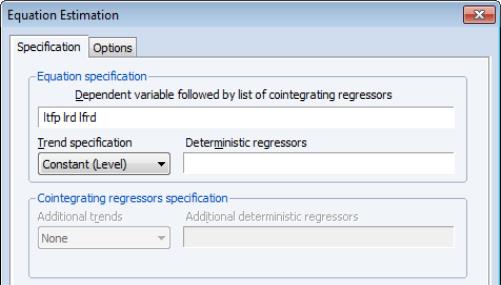
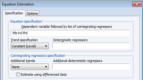
To begin, display the panel cointegrating equation dialog, and fill out the top portion of the dialog as depicted below:
Following KCC, we assume a fixed effect specification with LTFP as the dependent variable and LRD and LFRD as the cointegrating regressors. To handle the fixed effect we specify a in the drop-down menu.
The default panel cointegration estimation method using corresponds to the estimates in Table 4(i) of KCC, so we leave those settings unchanged.
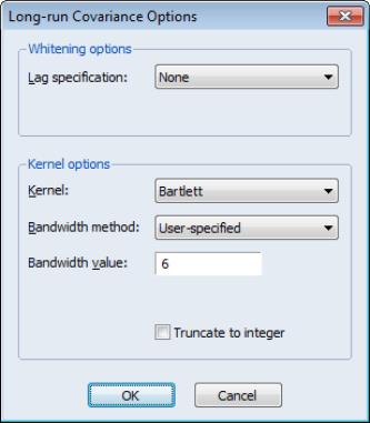
To match the KCC estimates, we click on button to display the long-run covariance settings, and change the by setting a user-specified bandwidth value of 6:
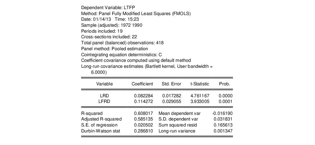
Click on to accept the changes. Since we wish to estimate the equation using the default coefficient covariances, we simply click on again to estimate the equation using the specified settings. EViews estimates the equation and displays the results:
The top portion of the dialog displays the estimation method and information about the sample employed in estimation. Just below the sample information EViews shows that the estimates are based on pooled estimation using only a constant as the cross-section specific trend regressor. The coefficient covariances are computed using the default settings, and the long-run covariances used a Bartlett kernel with the user-specified bandwidth.
The middle section shows the coefficient estimates, standard errors, and t-statistics, which differ a bit from the results in KCC Table 4(i), as KCC report estimates for a slightly different model. As in KCC, both R&D variables, LRD and LFRD are positively related to LTFP, and the coefficients are statistically significant.
The bottom portion of the output shows various summary statistics. Note in particular, the reported “Long-run variance” which shows

, the estimated long-run average variance of

conditional on

, obtained from the DOLS residuals. The square root of this variance, 0.0367, is somewhat higher than the “S.E. of the regression” value of 0.0205, which is based on the ordinary estimator of the residual variance.
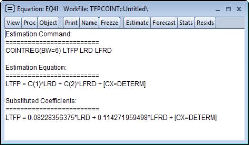
Clicking shows the commands used to estimate the equation, along with a text representation of the long-run relationship:
Note the “[CX=DETERM]” component which shows that there are additional heterogeneous trend terms in the relationship (in this case the fixed effects). The presence of this term instructs EViews to use this information when constructing models, and when computing fits and forecasts.
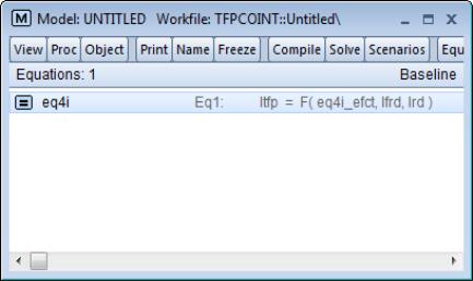
Suppose, for example, we select from our estimated equation.EViews will create a model object containing the equation results:
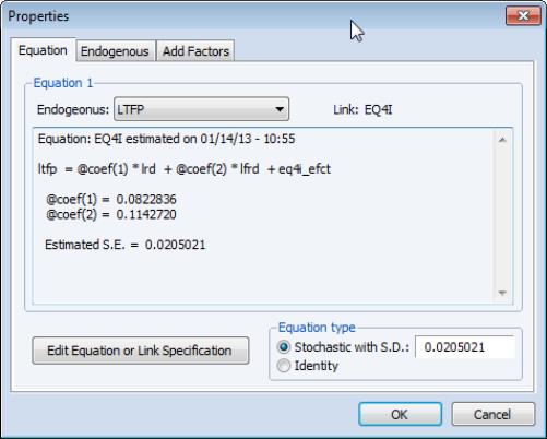
Notice the presence of EQ4I_EFCT in the model equation and in the workfile. Double-clicking on EQ4I in the model object displays the equation:
Notice that we have replaced the deterministic components “[CX=DETERM]” in the equation specification with the fitted values in the series EQ4I_EFCT. In this case EQ4I_EFCT just holds the estimated fixed effects, but more generally it will hold the fitted values for the deterministic terms in your regression.
To estimate the model using DOLS, we again display the equation dialog, fill out the top portion as before:
and change the to To match the settings in KCC, we set the to , and specify the lags and leads, with 2 lags and 1 lead:
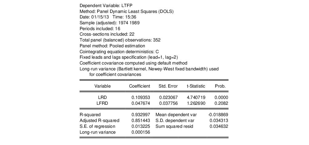
Click on OK to estimate the equation using the default covariance method. EViews will display the results:
Again, the top portion of the dialog shows the estimation method, sample, and information about settings employed in estimation. Note in particular that the default coefficient covariance matrix computation uses an estimator of the long-run variance computed using a Bartlett kernel and fixed Newey-West bandwidth.
The long-run coefficients, standard errors, and t-statistics are close to their counterparts in KCC Table 5(i).
We may contrast these results to the group-mean estimates of the same specifications. The group-mean FMOLS results may be obtained by calling up the original FMOLS equation and selecting in the drop-down menu. The group-mean FMOLS coefficient results are given by:
which differ markedly from the pooled estimates, suggesting that heterogeneity in the cointegrating equation or the long-run covariances may be important. Likewise, the corresponding group-mean DOLS results,
differ by a fair amount from the pooled results.


 , the estimated long-run average variance of
  conditional on
  , obtained from the DOLS residuals. The square root of this variance, 0.0367, is somewhat higher than the “S.E. of the regression” value of 0.0205, which is based on the ordinary estimator of the residual variance.