Forecasting with ARMA Errors
Forecasting from equations with ARMA components involves some additional complexities. When you use the AR or MA specifications, you will need to be aware of how EViews handles the forecasts of the lagged residuals which are used in forecasting.
Structural Forecasts
By default, EViews will forecast values for the residuals using the estimated ARMA structure, as described below.
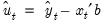
For some types of work, you may wish to assume that the ARMA errors are always zero. If you select the structural forecast option by checking , EViews computes the forecasts assuming that the errors are always zero. If the equation is estimated without ARMA terms, this option has no effect on the forecasts.
Forecasting with AR Errors
For equations with AR errors, EViews adds forecasts of the residuals from the equation to the forecast of the structural model that is based on the right-hand side variables.
In order to compute an estimate of the residual, EViews requires estimates or actual values of the lagged residuals. For the first observation in the forecast sample, EViews will use pre-sample data to compute the lagged residuals. If the pre-sample data needed to compute the lagged residuals are not available, EViews will adjust the forecast sample, and backfill the forecast series with actual values (see the discussion of
“Adjustment for Missing Values”).
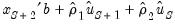
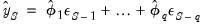
If you choose the option, both the lagged dependent variable and the lagged residuals will be forecasted dynamically. If you select , both will be set to the actual lagged values. For example, consider the following AR(2) model:
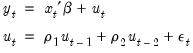 | (25.9) |
Denote the fitted residuals as
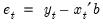
, and suppose the model was estimated using data up to

. Then, provided that the

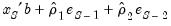
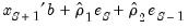
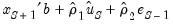
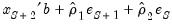
values are available, the static and dynamic forecasts for
, are given by:
where the residuals
are formed using the forecasted values of

. For subsequent observations, the dynamic forecast will always use the residuals based upon the multi-step forecasts, while the static forecast will use the one-step ahead forecast residuals.
Forecasting with MA Errors
In general, you need not concern yourselves with the details of MA forecasting, since EViews will do all of the work for you. However, for those of you who are interested in the details of dynamic forecasting, the following discussion should aid you in relating EViews results with those obtained from other sources.
We begin by noting that the key step in computing forecasts using MA terms is to obtain fitted values for the innovations in the pre-forecast sample period. For example, if you are performing dynamic forecasting of the values of

, beginning in period

, with a simple MA(

) process:
 | (25.10) |
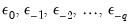
you will need values for the pre-forecast sample innovations,

. Similarly, constructing a static forecast for a given period will require estimates of the

lagged innovations at every period in the forecast sample.
If your equation is estimated with backcasting turned on, EViews will perform backcasting to obtain these values. If your equation is estimated with backcasting turned off, or if the forecast sample precedes the estimation sample, the initial values will be set to zero.
Backcast Sample
The first step in obtaining pre-forecast innovations is obtaining estimates of the pre-
estimation sample innovations:
. (For notational convenience, we normalize the start and end of the estimation sample to

and

, respectively.)
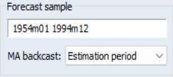
EViews offers two different approaches for obtaining estimates—you may use the dropdown menu to choose between the default and the methods.
The method uses data for the estimation sample to compute backcast estimates. Then as in estimation (
“Initializing MA Innovations”), the

values for the innovations
beyond the estimation sample are set to zero:
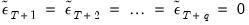 | (25.11) |
EViews then uses the unconditional residuals to perform the backward recursion:
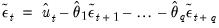 | (25.12) |
for
to obtain the pre-estimation sample residuals. Note that absent changes in the data, using produces pre-forecast sample innovations that match those employed in estimation (where applicable).
The method offers different approaches for dynamic and static forecasting:
• For dynamic forecasting, EViews applies the backcasting procedure using data from the beginning of the estimation sample to either the beginning of the forecast period, or the end of the estimation sample, whichever comes first.
• For static forecasting, the backcasting procedure uses data from the beginning of the estimation sample to the end of the forecast period.
For both dynamic and static forecasts, the post-backcast sample innovations are initialized to zero and the backward recursion is employed to obtain estimates of the pre-estimation sample innovations. Note that does not guarantee that the pre-sample forecast innovations match those employed in estimation.
Pre-Forecast Innovations
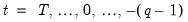
Given the backcast estimates of the pre-estimation sample residuals, forward recursion is used to obtain values for the pre-forecast sample innovations.
For dynamic forecasting, one need only obtain innovation values for the

periods prior to the start of the forecast sample; all subsequent innovations are set to zero. EViews obtains estimates of the pre-sample

using the recursion:
 | (25.13) |
for
, where

is the beginning of the forecast period
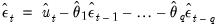
Static forecasts perform the forward recursion through the
end of the forecast sample so that innovations are estimated through the last forecast period. Computation of the static forecast for each period uses the

lagged estimated innovations. Extending the recursion produces a series of one-step ahead forecasts of both the structural model and the innovations.
Additional Notes
Note that EViews computes the residuals used in backcast and forward recursion from the observed data and estimated coefficients. If EViews is unable to compute values for the unconditional residuals

for a given period, the sequence of innovations and forecasts will be filled with NAs. In particular, static forecasts must have valid data for both the dependent and explanatory variables for all periods from the beginning of estimation sample to the end of the forecast sample, otherwise the backcast values of the innovations, and hence the forecasts will contain NAs. Likewise, dynamic forecasts must have valid data from the beginning of the estimation period through the start of the forecast period.
Example
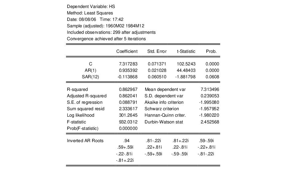
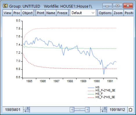
As an example of forecasting from ARMA models, consider forecasting the monthly new housing starts (HS) series. The estimation period is 1959M01–1984M12 and we forecast for the period 1985M01–1991M12. We estimated the following simple multiplicative seasonal autoregressive model,
hs c ar(1) sar(12)
yielding:
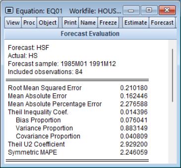
To perform a dynamic forecast from this estimated model, click on the equation toolbar, enter “1985m01 1991m12” in the Forecast sample field, then select and unselect . The forecast evaluation statistics for the model are shown below:
The large variance proportion indicates that the forecasts are not tracking the variation in the actual HS series. To plot the actual and forecasted series together with the two standard error bands, you can type:
smpl 1985m01 1991m12
plot hs hs_f hs_f+2*hs_se hs_f-2*hs_se
where HS_F and HS_SE are the forecasts and standard errors of HS.
As indicated by the large variance proportion, the forecasts track the seasonal movements in HS only at the beginning of the forecast sample and quickly flatten out to the mean forecast value.