Robust Standard Errors
In the linear least squares regression model, the variance-covariance matrix of the estimated coefficients may be written as:
 | (21.8) |
where

.
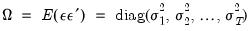
If the error terms,

, are homoskedastic and uncorrelated so that
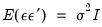
, the covariance matrix simplifies to the familiar expression
 | (21.9) |
By default, EViews estimates the coefficient covariance matrix under the assumptions underlying
Equation (21.9), so that
 | (21.10) |
and
 | (21.11) |
where

is the standard degree-of-freedom corrected estimator of the residual variance.
We may instead employ robust estimators of the coefficient variance

which relax the assumptions of heteroskedasticity and/or zero correlation. Broadly speaking, EViews offers three classes of robust variance estimators that are:
• Robust in the presence of heteroskedasticity. Estimators in this first class are termed Heteroskedasticity Consistent (HC) Covariance estimators.
• Robust in the presence of correlation between observations in different groups or clusters. This second class consists of the family of Cluster Robust (CR) variance estimators.
• Robust in the presence of heteroskedasticity and serial correlation. Estimators in the third class are referred to as Heteroskedasticity and Autocorrelation Consistent Covariance (HAC) estimators.
All of these estimators are special cases of
sandwich estimators of the coefficient covariances. The name follows from the structure of the estimators in which different estimates of

are sandwiched between two instances of an outer moment matrix.
It is worth emphasizing all three of these approaches alter the estimates of the coefficient standard errors of an equation but not the point estimates themselves.
Lastly, our discussion here focuses on the linear model. The extension to nonlinear regression is described in
“Nonlinear Least Squares”.
Heteroskedasticity Consistent Covariances
First, we consider coefficient covariance estimators that are robust to the presence of heteroskedasticity.
We divide our discussion of HC covariance estimation into two groups: basic estimators, consisting of White (1980) and degree-of-freedom corrected White (Davidson and MacKinnon 1985), and more general estimators that account for finite samples by adjusting the weights given to residuals on the basis of leverage (Long and Ervin, 2000; Cribari-Neto and da Silva, 2011).
Basic HC Estimators
White (1980) derives a heteroskedasticity consistent covariance matrix estimator which provides consistent estimates of the coefficient covariances in the presence of (conditional) heteroskedasticity of unknown form, where
 | (21.12) |
Recall that the coefficient variance in question is
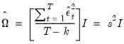
Under the basic White approach. we estimate the central matrix

using either the d.f. corrected form
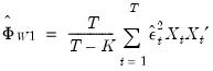 | (21.13) |
or the uncorrected form
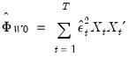 | (21.14) |
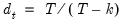
where

are the estimated residuals,

is the number of observations,

is the number of regressors, and

is the conventional degree-of-freedom correction.
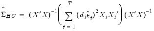
The estimator of

is then used to form the heteroskedasticity consistent coefficient covariance estimator. For example, the degree-of-freedom White heteroskedasticity consistent covariance matrix estimator is given by
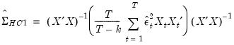 | (21.15) |
Estimates using this approach are typically referred to as White or Huber-White or (for the d.f. corrected case) White-Hinkley covariances and standard errors.
Example
To illustrate the computation of White covariance estimates in EViews, we employ an example from Wooldridge (2000, p. 251) of an estimate of a wage equation for college professors. The equation uses dummy variables to examine wage differences between four groups of individuals: married men (MARRMALE), married women (MARRFEM), single women (SINGLEFEM), and the base group of single men. The explanatory variables include levels of education (EDUC), experience (EXPER) and tenure (TENURE). The data are in the workfile “Wooldridge.WF1”.
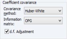
To select the White covariance estimator, specify the equation as before, then select the tab and select in the drop-down. You may, if desired, use the checkbox to remove the default , but in this example, we will use the default setting. (Note that the combo setting is not important in linear specifications).
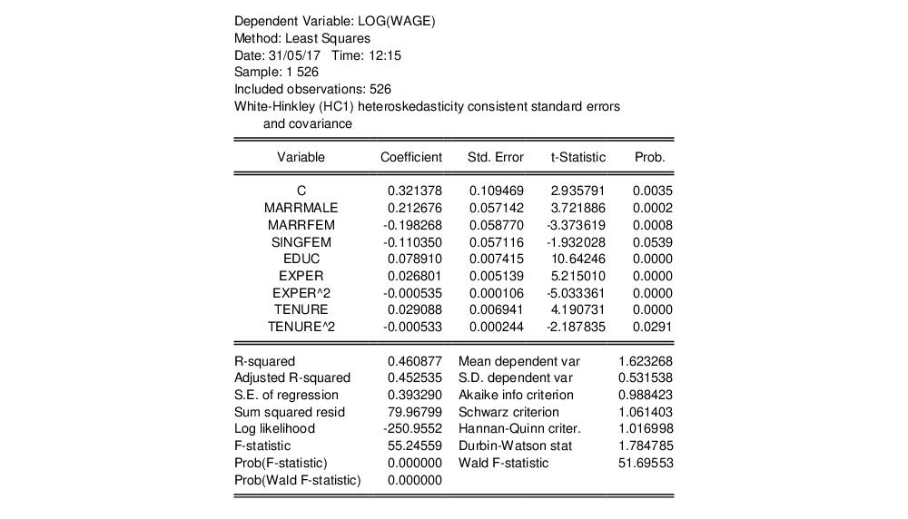
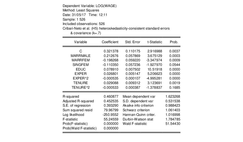
The output for the robust covariances for this regression are shown below:
As Wooldridge notes, the heteroskedasticity robust standard errors for this specification are not very different from the non-robust forms, and the test statistics for statistical significance of coefficients are generally unchanged. While robust standard errors are often larger than their usual counterparts, this is not necessarily the case, and indeed in this example, there are some robust standard errors that are smaller than their conventional counterparts.
Notice that EViews reports both the conventional residual-based F-statistic and associated probability and the robust Wald test statistic and p-value for the hypothesis that all non-intercept coefficients are equal to zero.
Recall that the familiar residual F-statistic for testing the null hypothesis depends only on the coefficient point estimates, and not their standard error estimates, and is valid only under the maintained hypotheses of no heteroskedasticity or serial correlation. For ordinary least squares with conventionally estimated standard errors, this statistic is numerically identical to the Wald statistic. When robust standard errors are employed, the numerical equivalence between the two breaks down, so EViews reports both the non-robust conventional residual and the robust Wald F-statistics.
EViews reports the robust F-statistic as the Wald F-statistic in equation output, and the corresponding p-value as Prob(Wald F-statistic). In this example, both the non-robust F-statistic and the robust Wald show that the non-intercept coefficients are jointly statistically significant.
Alternative HC Estimators
The two familiar White covariance estimators described in
“Basic HC Estimators” are two elements of a wider class of HC methods (Long and Ervin, 2000; Cribari-Neto and da Silva, 2011).
This general class of heteroskedasticity consistent sandwich covariance estimators may be written as:
 | (21.16) |
where

are observation-specific weights that are chosen to improve finite sample performance.
The various members of the class are obtained through different choices for the weights. For example, the standard White and d.f. corrected White estimators are obtained by setting

and
for all

, respectively.
EViews allows you to estimate your covariances using several choices for

. In addition to the standard White covariance estimators from above, EViews supports the bias-correcting HC2, pseudo-jackknife HC3 (MacKinnon and White, 1985), and the leverage weighting HC4, HC4m, and HC5 (Cribari-Neto, 2004; Cribaro-Neto and da Silva, 2011; Cribari-Neto, Souza, and Vasconcellos, 2007 and 2008).
The weighting functions for the various HC estimators supported by EViews are provided below:
| |
HC0 – White | 1 |
HC1 – White with d.f. correction | |
HC2 – bias corrected | |
HC3 – pseudo-jackknife | |
HC4 – relative leverage | |
HC4m | |
HC5 | |
User – user-specified | arbitrary |
where
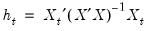
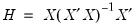
are the diagonal elements of the familiar “hat matrix”

.
Note that the HC0 and HC1 methods correspond to the basic White estimators outlined earlier.
Note that HC4, HC4m, and HC5 all depend on an exponential discounting factor

that differs across methods:
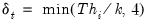
• For HC4,
is a truncated function of the ratio between

and the mean

(Cribari-Neto, 2004; p. 230).
• For HC4m,
where

and

are pre-specified parameters (Cribari-Neto and da Silva, 2011). Following Cribari-Neto and da Silva,
EViews chooses default values of

and

.
• For HC5,
is similar to the HC4 version of

, but with observation specific truncation that depends on the maximal leverage and a pre-specified parameter

(Cribari-Neto, Souza, and Vasconcellos, 2007 and 2008).
EViews employs a default value of

.
Lastly, to allow for maximum flexibility, EViews allows you to provide user-specified

in the form of a series containing those values.
Each of the weight choices modifies the effects of high leverage observations on the calculation of the covariance. See Cribari-Neto (2004), Cribari-Neto and da Silva (2011), and Cribari-Neto, Souza, and Vasconcellos (2007, 2008) for discussion of the effects of these choices.
Note that the full set of HC estimators is only available for linear regression models. For nonlinear regression models, the leverage based methods are not available and only user-specified may be computed.
Example
To illustrate the use of the alternative HC estimators, we continue with the Wooldridge example (
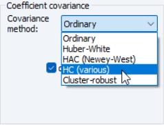
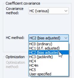
“Example”) considered above. We specify the equation variables as before, then select the tab and click on the drop-down and select :
The dialog will change to show you additional options for selecting the :
Note that the and items replicate the option from the original dropdown and are included in this list for completeness. If desired, change the method from the default , and if necessary, specify values for the parameters. For example, if you select User-specified, you will be prompted to provide the name of a series in the workfile containing the values of the weights

.
Continuing with our example, we use the dropdown to select the method, and retain the default value

. Click on to estimate the model with these settings producing the following results:
The effects on statistical inference resulting from a different HC estimator are minor, though the quadratic effect of TENURE is no longer significant at conventional test levels.
Cluster-Robust Covariances
In many settings, observations may be grouped into different groups or “clusters” where errors are correlated for observations in the same cluster and uncorrelated for observations in different clusters. EViews offers support for consistent estimation of coefficient covariances that are robust to either one and two-way clustering.
We begin with a single clustering classifier and assume that
 | (21.17) |
for all

and

in the same cluster, and all

and

that are in different clusters. If we assume that the number of clusters

goes to infinity, we may compute a cluster-robust (CR) covariance estimate that is robust to both heteroskedasticity and to within-cluster correlation (Liang and Zeger, 1986; Wooldridge, 2003; Cameron and Miller, 2015).
As with the HC and HAC estimators, the cluster-robust estimator is based upon a sandwich form with an estimator the central matrix

:
 | (21.18) |
where

is the

matrix of regressors for the

observations in the
g-th cluster,

is a

vector of errors, and

is a

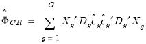
diagonal matrix of weights for the observations in the cluster. The resulting family of CR variance estimators is given by:
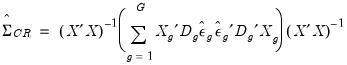 | (21.19) |
The EViews supported weighting functions for the various CR estimators are analogues to those available for HC estimation:
| |
CR0 – Ordinary | 1 |
CR1 – finite sample corrected (default) | |
CR2 – bias corrected | |
CR3 – pseudo-jackknife | |
CR4 – relative leverage | |
CR4m | |
CR5 | |
User – user-specified | arbitrary |
where

are the diagonal elements of
. For further discussion and detailed definitions of the discounting factor

in the various methods, see
“Alternative HC Estimators”. See Cameron and Miller (CM 2015, p. 342) for discussion of bias adjustments in the context of cluster robust estimation.
Note that the EViews CR3 differs slightly from the CR3 described by CM in not including the

factor, and that we have defined the CR4, CR4m and CR5 estimators which employ weights that are analogues to those defined for HC covariance estimation.
We may easily extend the robust variance calculation to two-way clustering to handle cases where observations are correlated within two different clustering dimensions (Petersen 2009, Thompson 2011, Cameron, Gelbach, and Miller 2015).
It is easily shown that the variance estimator for clustering by

and

may be written as:
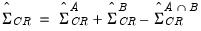 | (21.20) |
where the

is used to indicate the estimator obtained assuming clustering along the given dimension. Thus, the estimator is formed by adding the covariances obtained by clustering along each of the two dimensions individually, and subtracting off the covariance obtained by defining clusters for the intersection of the two dimensions.
Note that EViews does not perform the eigenvalue adjustment in cases where the resulting estimate is not positive semidefinite.
If you elect to compute cluster-robust covariance estimates, EViews will adjust the
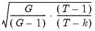
t-statistic probabilities in the main estimation output to account for the clustering and will note this adjustment in the output comments. Following Cameron and Miller (CM, 2015), the probabilities are computed using the
t-distribution with

degrees-of-freedom in the one-way cluster case, and by
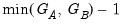
degrees-of-freedom under two-way clustering. Bear in mind that CM note that even with these adjustments, the tests tend to overreject the null.
Furthermore, when cluster-robust covariances are computed, EViews will not display the residual-based F-statistic for the test of significance of the non-intercept regressors. The robust Wald-based F-statistic will be displayed.
Example
We illustrate the computation of cluster-robust covariance estimation in EViews using the test data provided by Petersen via his website:
The data are provided as an EViews workfile “Petersen_cluster.WF1”. There are 5000 observations on four variables in the workfile, the dependent variable Y, independent variable X, and two cluster variables, a firm identifier (FIRMID), and time identifier (YEAR). There are 500 firms, and 10 periods in the balanced design.
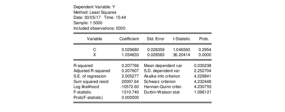
First, create the equation object in EViews by selecting or from the main menu, or simply type the keyword equation in the command window. Enter, the regression specification “Y C X” in the edit field, and click on to estimate the equation using standard covariance settings.
The results of this estimation are given below:
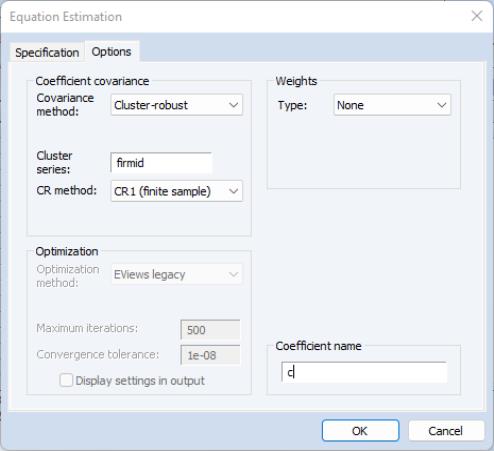
Next, to estimate the equation with FIRMID cluster-robust covariances, click on the button on the equation toolbar to display the estimation dialog, and then click on the tab to show the options.
Select in the dropdown, enter “FIRMID” in the edit field, and select a . Here, we choose the method which employs a simple d.f. style adjustment to the basic cluster covariance estimate. Click on to estimate the equation using these settings.
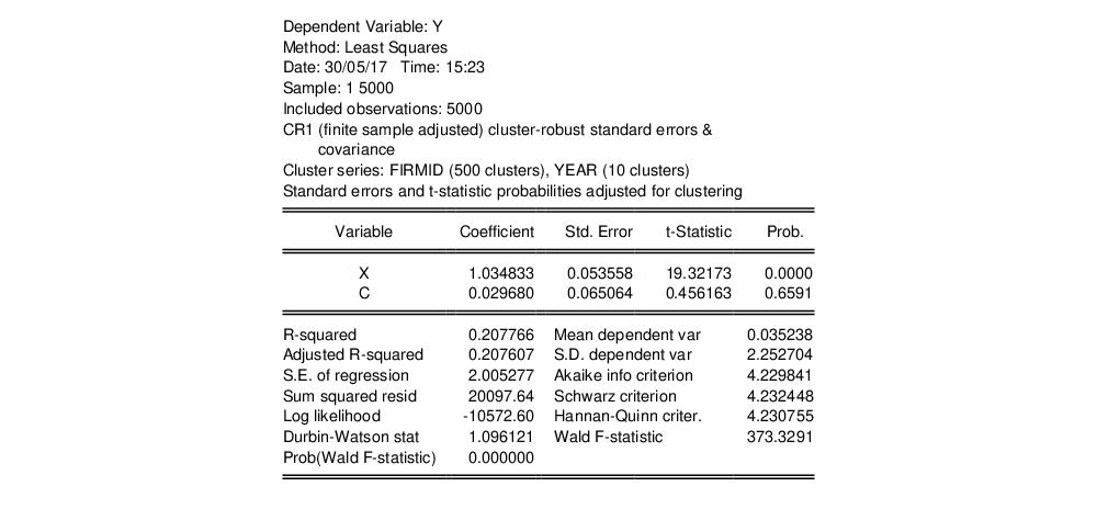
The results are displayed below:
The top portion of the equation output describes both the cluster method (CR1) and the cluster series (FIRMID), along with the number of clusters (500) observed in the estimation sample. In addition, EViews indicates that the reported coefficient standard errors, and
t-statistic probabilities have been adjusted for the clustering. As noted earlier, the probabilities are computed using the
t-distribution with

degrees-of-freedom.
Note also that EViews no longer displays the ordinary F-statistic and associated probability, but instead shows the robust Wald F-statistic and probability.
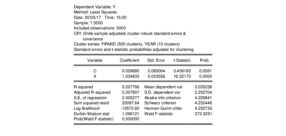
For two-way clustering, we create an equation with the same regression specification, click on the tab, and enter the two cluster series identifiers “FIRMID YEAR” in the edit field. Leaving the remaining options at their current settings, click on to compute and display the estimation results:
The output shows that the cluster-robust covariance computation is now based on two-way clustering using the 500 clusters in FIRMID and the 10 clusters in YEAR. The
t-statistic probabilities are now based on the
t-distribution with
degrees-of-freedom.
Notice in all of these examples that the coefficient point estimates and basic fit measures are unchanged. The only changes in results are in the estimated standard errors, and the associated t-statistics, probabilities, and the F-statistics and probabilities.
Lastly, we note that the standard errors and corresponding statistics in the EViews two-way results differ slightly from those reported on the Petersen website. These differences appear to be the result of slightly different finite sample adjustments in the computation of the three individual matrices used to compute the two-way covariance. When you select the CR1 method, EViews adjusts each of the three matrices using the CR1 finite sample adjustment; Petersen’s example appears to apply CR1 to the one-way cluster covariances, while the joint two-way cluster results are computing using CR0.
HAC Consistent Covariances (Newey-West)
The White covariance matrix described above assumes that the residuals of the estimated equation are serially uncorrelated.
Newey and West (1987b) propose a covariance estimator that is consistent in the presence of both heteroskedasticity and autocorrelation (HAC) of unknown form, under the assumption that the autocorrelations between distant observations die out. NW advocate using kernel methods to form an estimate of the long-run variance,
.
EViews incorporates and extends the Newey-West approach by allowing you to estimate the HAC consistent coefficient covariance estimator given by:
 | (21.21) |
where

is any of the LRCOV estimators described in
Appendix F. “Long-run Covariance Estimation”.
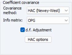
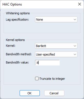
To use the Newey-West HAC method, select the tab and select in the drop-down. As before, you may use the checkbox to remove the default .
Press the button to change the options for the LRCOV estimate.
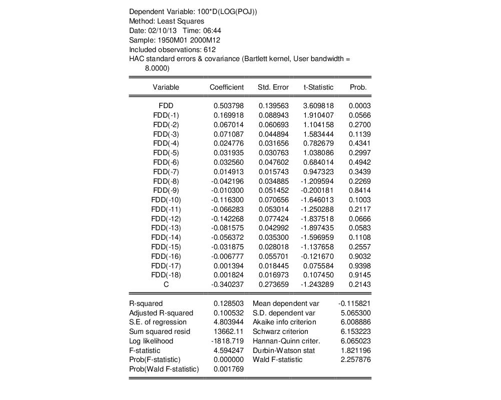
We illustrate the computation of HAC covariances using an example from Stock and Watson (2007, p. 620). In this example, the percentage change of the price of orange juice is regressed upon a constant and the number of days the temperature in Florida reached zero for the current and previous 18 months, using monthly data from 1950 to 2000 The data are in the workfile “Stock_wat.WF1”.
Stock and Watson report Newey-West standard errors computed using a non pre-whitened Bartlett Kernel with a user-specified bandwidth of 8 (note that the bandwidth is equal to
one plus what Stock and Watson term the “truncation parameter”

).
The results of this estimation are shown below:
Note in particular that the top of the equation output documents the use of HAC covariance estimates along with relevant information about the settings used to compute the long-run covariance matrix.
The HAC robust Wald p-value is slightly higher than the corresponding non-robust F-statistic p-value, but are significant at conventional test levels.