VARs With Linear Constraints
The basic

-variable VAR(
p) specification has

coefficients so that even moderate sized VARs require estimation of a large number of parameters. When VARs are applied to macroeconomic data with limited sample sizes, model over-parameterization is a frequent problem as there are too few observations to estimate precisely the VAR parameters.
EViews offers two approaches to handling this over-parameterization problem:
• Alternately, you may reduce the number of free parameters by imposing linear constraints on the elements of

.
We outline here EViews’s tools for imposing linear restrictions. Note that we previously explored a variant of the constraint approach where specification of the VAR lag structure using multiple lag pairs sets a subset of lag matrices

to zero (
“Estimating a VAR in EViews”). In contrast, the more general methods described in this section permit finely targeted restriction on the parameters, allowing us to incorporate
a priori information about the parameters of the model which does not fit into the lag exclusion framework.
Briefly, to echo the discussion in Lütkepohl (2006), suppose we have linear restrictions of the form:
 | (44.14) |
where

is the
vector of VAR coefficients,

is a
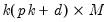
restriction matrix,

is a

vector of unconstrained parameters and

is a

vector of known constants.
Note that while this is not the most common form for expressing linear restrictions, the conventional (

) form of linear restrictions,

, may readily be transformed to the (

) form (see Lütkepohl 2006, p. 195).
Substituting
Equation (44.14) into
Equation (44.5) produces an unrestricted regression specification
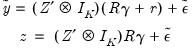 | (44.15) |
where
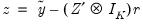
.
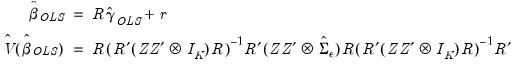
The OLS estimator for

is given by
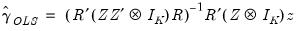 | (44.16) |
and a estimator of the variance of

is given by
 | (44.17) |
for the consistent estimator
 | (44.18) |
Note that we employ the unadjusted residual variance matrix estimator since the presence of restrictions produces ambiguity in the finite sample correction.
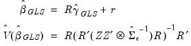
Efficiency gains may be realized by accounting for the contemporaneous correlation in the errors. For

, a consistent estimator of

the estimated GLS estimator is given by
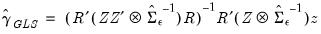 | (44.19) |
Note that any consistent estimator for

may be employed. By default, EViews will iterate over estimates of

and the

obtained using the current residuals until convergence, or the maximum number of iterations is reached. Alternately, you may elect to perform only a single GLS iteration.
A consistent estimator of the coefficient covariance is given by
 | (44.20) |
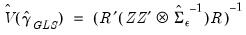
The corresponding estimators and covariances for the full coefficient vector

are then
 | (44.21) |
and
 | (44.22) |
Bear in mind that by construction,

has reduced rank.
Estimating a VAR with Linear Restrictions in EViews
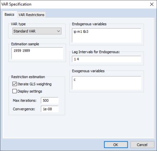
Select or type var in the command window to display the estimation dialog.
The
Basics tab of the VAR Specification dialog outlines the basic specification, and should be filled out as for a basic specification (
“Estimating a VAR in EViews”).
Click on the VAR Restrictions tab to specify your restrictions:
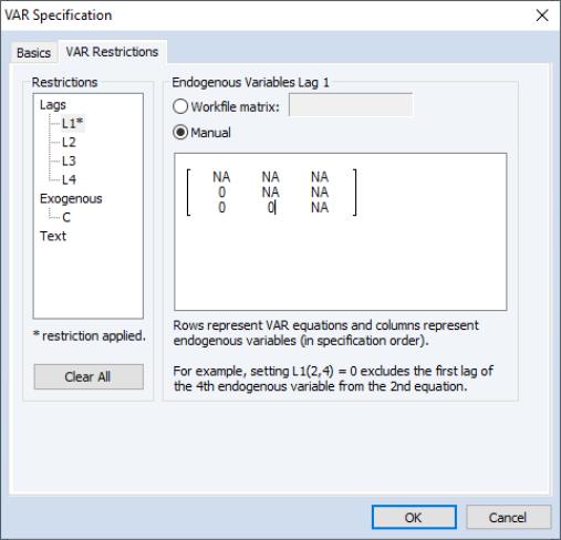
The section on the left should be used to select the VAR elements that you wish to restrict. You may click on the entries for the lag matrices (, , , ) and the vectors of coefficients associated with each exogenous variable () to select an element to restrict. The right side of the dialog will change to show the current settings for the selected element.
• If the method is selected, you will place restrictions on the selection by editing its matrix representation in the dialog (rows of the matrix represent VAR equations while columns represent the endogenous variable). The ordering of the matrix elements follows the order of the endogenous variables in the original specification. Elements of the matrix or vector that are NA will be estimated while the remaining elements will be restricted to the specified value.
Here, we have selected the matrix for the first lag of the endogenous variables () and set two elements to zero so that the lag of the first endogenous variable has no effect on the second and third endogenous variables.
• If the method is selected, you should enter the name of a matrix object in the workfile containing the restriction matrix for the selection. The matrix should be of the correct dimension and should have NAs for unrestricted elements and numeric values for restricted elements.
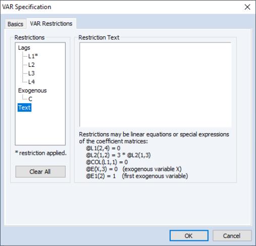
In settings where restricting a large number individual elements is inconvenient, or where you wish to impose restrictions across lag or exogenous variable coefficients, you may find it more convenient to specify restrictions using text expressions. In this case, click on the node of the tree to display the edit field.
Text expressions allow you to use a function-like syntax to employ text to specify restrictions on one or more matrix elements. The text restrictions will use the following “@” keywords that you may use to refer to individual coefficient matrix elements,
@l#(r, c) | Element (r, c) of the lag # coefficient matrix. |
@e#(r) | Element r of the exogenous variable # coefficient vector. |
@e(X, r) | Element r of the exogenous variable X coefficient vector |
Note that in this syntax, the canonical names (“L#”, “E#”, “E(X)”) that refer to lag matrices and exogenous variable vectors are preceded by “@” to avoid ambiguity.
For example, we may have:
@L1(1,1) = 0
@L2(2,2) = @L1(3,3) / 2
@L2(1,1) + @L4(2,1) = 1
@E(C, 1) = 0
@E(X, 2) = @E(C, 2)
@E1(1) + @E1(2) = 1
In addition, you may use text expressions to refer to parts of lag coefficient matrices and to impose specialized restrictions,
| Restricts all elements of matrix W similar to a pattern matrix. Element ordering matches the vectorization of the matrix, i.e., the elements of the first column, followed by the second column, followed by the third column, etc. |
@diag(W) | Restricts W to be a diagonal matrix, i.e., off-diagonal elements are zero. The diagonal elements are unrestricted. |
@diag(W) = n | Restricts W to be a diagonal matrix with elements on the diagonal restricted to be n. |
@lower(W) | Restricts W to be a lower triangular matrix, i.e., elements above the diagonal are zero. |
@unitlower(W) | Restricts W to be a unit lower triangular matrix, i.e., elements above the diagonal are zero and elements on the diagonal are one. |
@upper(W) | Restricts W to be an upper triangular matrix, i.e., elements below the diagonal are zero. |
@unitupper(W) | Restricts W to be a unit upper triangular matrix, i.e., elements below the diagonal are zero and elements on the diagonal are one. |
@row(W, r) = n | Restricts the elements in row r of W to be n. |
@col(W, c) = n | Restricts the elements in column c of W to be n. |
where

is a reference to a canonical matrix name (
e.g., “L1”, “L3”).
For example:
@row(L1, 2) = 0
@lower(L5)
You may specify your restrictions with any combination of direct assignment or text expressions. EViews will analyze the specification and determine if there are any restrictions that are incompatible.
If restrictions have been applied to any elements, the left side of the dialog will note this fact with the line of text “* restrictions applied”, and the button will be enabled. The button allows you to easily remove all of the current restrictions.
When restrictions have been applied, the tab of the dialog will change to offer additional options. In the newly displayed in the bottom left o the dialog, you will be prompted to specify the method of estimating your restricted coefficients:
In you do not select the option, EViews will estimate the parameters of the model using one-step GLS estimation. If you do select to specify the iteration and convergence properties of the estimation. To estimate with OLS, you may select and specify a of 0.
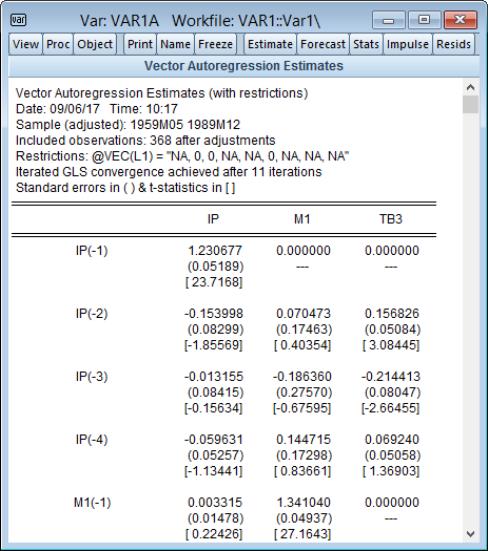
Estimation Output (Linear Restrictions)
Following estimation, EViews will display the results of restricted estimation. For the most part, the results are as described in
“Estimation Output”, but there are some differences of note.
First, the top of the estimation output shows that the VAR estimates were estimated with restrictions, and provides a text description of the restrictions. Here we see that in our illustration, we have placed zero restrictions on the first lag coefficients for IP in the M1 equation, and for IP and M1 in the TB3 equation.
Just below the restrictions specification, EViews displays information about the restricted estimation method. Here, we see that EViews estimated the VAR using iterated GLS and that the coefficients and GLS weight matrix converged after 11 iterations.
The coefficients display shows the full set of VAR coefficient estimates with restrictions imposed as appropriate. In cases, where the estimated standard error of the coefficient is zero, the display will show “---” and the t-statistic is suppressed.
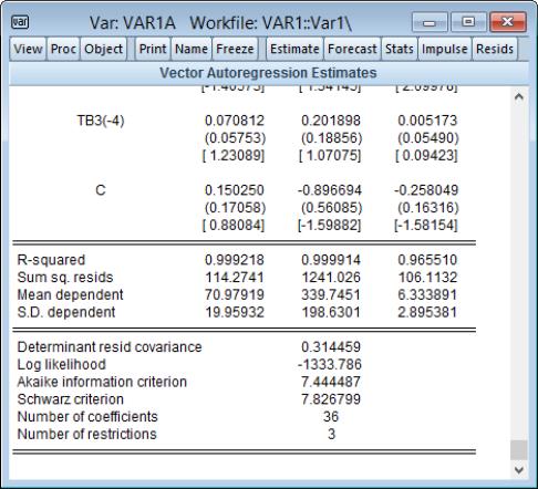
As for unrestricted VARs, the bottom of the output show additional information on the individual equations and summary statistics for the VAR as a whole:
As before, there are standard OLS regression summary statistics at the bottom of the column for the corresponding equation. Since linearly restricted VAR regression is not computed on an equation by equation basis, EViews only displays a subset of the equation specific statistics that are available for unrestricted VAR estimation.
The remaining output consists of summary statistics for the VAR system as a whole. These statistics include the determinant of the residual covariance (non-d.f. corrected), log-likelihood and associated information criteria, the number of coefficients, and number of restrictions.
 ,
,  ,
,  , ...
, ...