Example
As an example of using variable selection in EViews, we will estimate a model of hourly electricity spot prices. We will follow, in spirit, the analysis done in Uniejewski, Nowotarski and Weron (2016), estimating a model with a large number of candidate variables to try to perform a one day-ahead forecast of the spot price.
We have a workfile containing hourly data between 2015 and 2018 of the electricity spot price for a region in the United States, along with hourly electricity load data (how much electricity is used) and day-ahead load forecasts for the same region.
As a dependent variable we use the series TPRICE containing the deviation of the log of the spot price from the mean of the log of spot prices for the same hour.
We have a total of 107 search regressors:
• 3 days (72 hours) of lags of TPRICE (72)
• a single one week (168 hour) lag of TPRICE (1)
• the minimum TPRICE of the previous day, two days before and three days before (3)
• the maximum TPRICE of the previous day, two days before and three days before (3)
• the mean TPRICE of the previous day, two days before and three days before (3)
• log of electricity load for current hour, same hour previous day and same hour previous week (3)
• log of forecasted load for same hour next day (1)
• day of week dummy variables (set to zero for weekday holidays) (7)
• Interaction between dummy variables and log of load (y)
• Interaction between dummy variables and TPRICE (7)
These search regressions are stored in the group SEARCHREGS.
The model also has an always-included constant.
For this example we will model TPRICE at noon each day between January 1, 2015 and December 30, 2018, and will use those estimates to forecast TPRICE for December 31, 2018 —a one observation forecast.
Stepwise Example
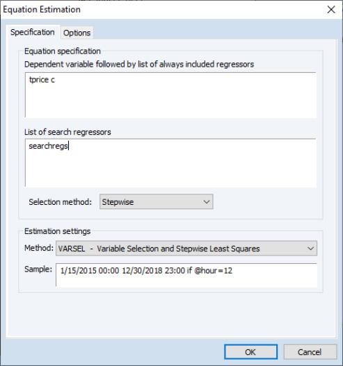
To begin, we’ll use a stepwise regression to select the most appropriate regressors. We click on to bring up the dialog, and then change the dropdown to .
• We enter “TPRICE C” in the first part of the , and then “SEARCHREGS” in the box.
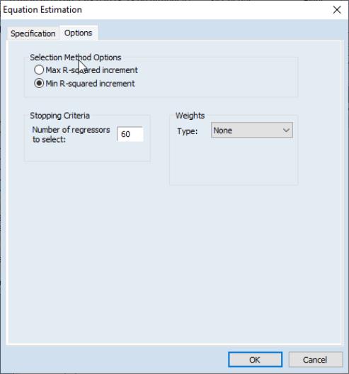
• We’ll leave the as , and keep the options on the tab at their default settings.
• Finally we set the sample to be the estimation dates we want, ensuring that only the noon observations are used.
Clicking performs the stepwise variable selection, and estimates the final model. The top portion of the output describes the selection process:
The final line issues a warning that the final estimation results shown use a different sample than that used during selection. This is because some of the search regressors contain NAs (due to lags in our case), and thus those observations are dropped from the selection process. However some of those variables were not selected, and so those observations can be re-included in the final estimation.
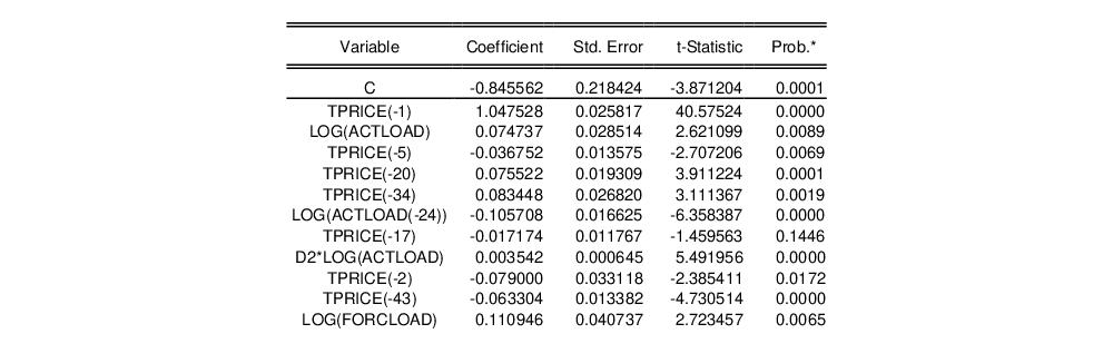
The middle part of the output (partially shown here) displays the selected variables, their coefficients, standard errors, t-statistics and probability values.
In this case a total of 54 of the 107 search regressors were selected.
The bottom of the output (partially shown) describes the selection process the stepwise regression undertook.
Swapwise Example
For a second estimation of the model, we will use the swapwise algorithm. We again click on to bring up the dialog, and fill in the variables and sample as before. We change the combo to .
Switching to the tab, we switch to and instruct EViews to find the best 60 regressors (which seems a reasonable number given the stepwise procedure’s selection of 54).
The output from this equation is similar to that of the first—the top portion displays a summary of the estimation, the middle section provides the estimation results, and the bottom portion displays the selection process.
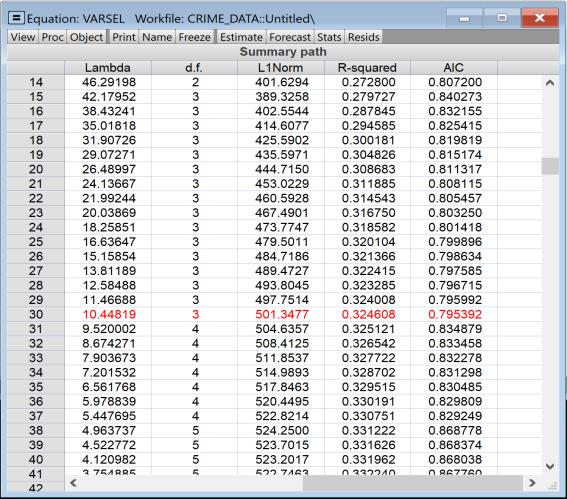
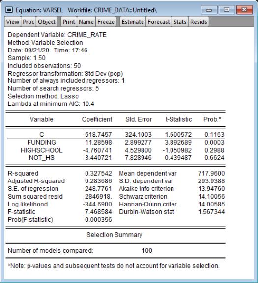
Auto-search/GETS Example
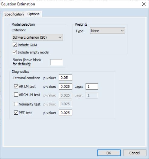
Our third estimation will use the Auto-search/GETS algorithm. On the page, change the to , and then click on the tab to alter some of the default settings. We’ll change the criteria used to decide between the final candidate models to the Schwarz criterion using the dropdown. We also elect to only use the AR LM test and PET tests as diagnostic tests during the path search.
The output from this estimation is similar to the previous two; the upper portion describes the selection method, the middle displays the final model’s coefficient estimates and associates statistics, and the bottom provides some small detail on the selection process. In contrast to the stepwise procedure, Auto-search has only selected 27 regressors.
Lasso Example
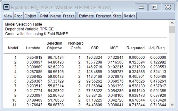
In this example employ Lasso to select a model for the electricity data. On the page, change the to ,
We leave the page settings at their default values, but click on the Cross-validation options button and change the K-fold to and the to 20. Click on OK to accept the and then click on to estimate the model using the specified settings.
The top of the main estimation output shows information about the Lasso estimation settings:
Among other things, EViews uses an automatic path determination to specify the
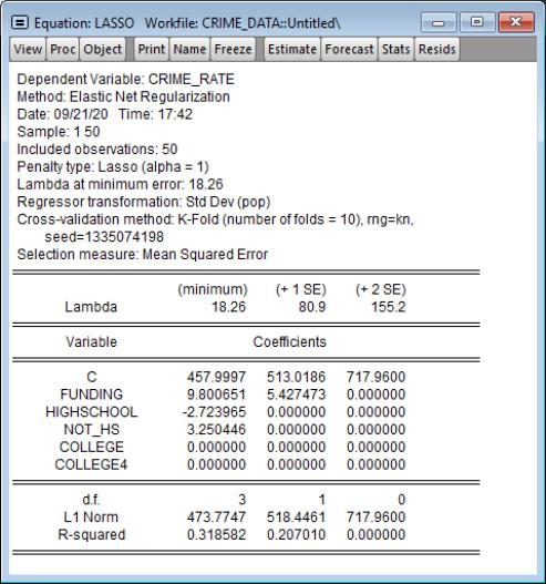
, and employs K-Fold cross-validation with a SMAPE objective to determine an optimal penalty. The optimal
is 0.002031.
The middle portion of the output shows the results for OLS estimation using the variables with non-zero coefficients in the Lasso estimation.
Below the OLS coefficients are the usual summary statistics:
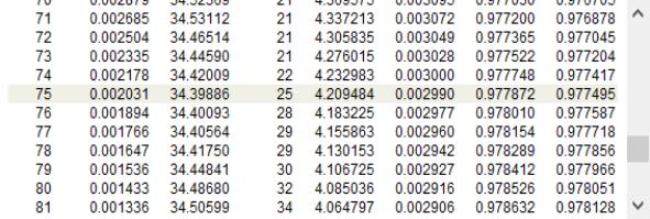
The bottom of the output reports that the cross-validation model selection compared 100 values of the penalty parameter. Lasso selects 24 regressors out of the 107 search regressors.
EViews also reminds you that the standard errors, p-values, and test results reported in this table are for OLS given the variables selected, and do not account for the randomness associated with Lasso variable selection.
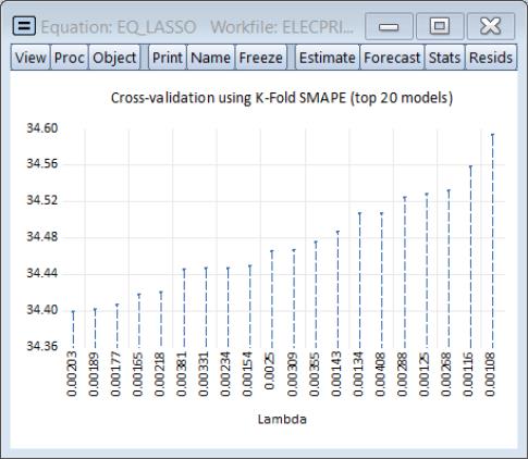
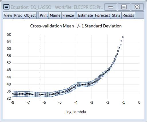
We may examine details of the model selection process by going to and choosing or . The display a graph of the models ranked from best to worst in order of the cross-validation statistic:
The view shows the cross-validation objective and other fit statistics in tabular form, ordered by value of the penalty. The optimal value will be highlighted.
Selecting , shows a graph of the full path of the cross-validation evaluation statistic:
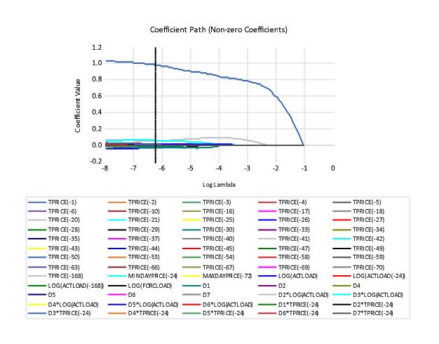
Under the menu EViews also offers views from elastic net estimation. Of particular interest is the view which (among other graphs) plots the (anywhere) non-zero coefficients against the lambda path: