Unit Root Tests with a Breakpoint
The use of unit root tests to distinguish between trend and difference stationary data has become an essential tool in applied research. Accordingly, EViews offers a variety of standard unit root tests, including augmented Dickey-Fuller (ADF), Phillips-Perron (PP), Elliot, Rothenberg, and Stock (ERS), Ng and Perron (NP), and Kwiatkowski, Phillips, Schmidt, and Shin (KPSS) tests (
“Unit Root Testing”).
However, as Perron (1989) points out, structural change and unit roots are closely related, and researchers should bear in mind that conventional unit root tests are biased toward a false unit root null when the data are trend stationary with a structural break. This observation has spurred development of a large literature outlining various unit root tests that remain valid in the presence of a break (see Hansen, 2001 for an overview).
EViews offers support for several types of modified augmented Dickey-Fuller tests which allow for levels and trends that differ across a single break date. You may compute unit root tests with a single break where:
• The break can occur slowly or immediately.
• The break consists of a level shift, a trend break, or both a shift and break.
• The break date is known, or the break date is unknown and estimated from the data.
• The data are non-trending or trending.
Background
We begin with a brief discussion of the specifications underlining the testing methodology. As always, our discussion is necessarily brief and we encourage you to consult the enclosed references for additional detail.
Our discussion follows the basic framework outlined in Perron (1989), Vogelsang and Perron (1998), Zivot and Andrews (1992), Banerjee et al. (1992) and others. For a useful overview of the literature, see Perron (2006). Note that our notation differs slightly from the above sources.
Break Variables
Before proceeding, it will be useful to define a few variables which allow us to characterize the breaks. Let

be an indicator function that takes the value 1 if the argument
is true, and 0 otherwise. Then the following variables are defined in terms of a specified break date
,
• An intercept break variable
 | (42.45) |
that takes the value 0 for all dates prior to the break, and 1 thereafter.
• A trend break variable
 | (42.46) |
which takes the value 0 for all dates prior to the break, and is a break date re-based trend for all subsequent dates.
• A one-time break dummy variable
 | (42.47) |
which takes the value of 1 only on the break date and 0 otherwise.
Note that following EViews convention, we define the break date as the first date for the new regime. This is in contrast to much of the literature which defines the break date as the last date of the previous regime.
The Model
Following Perron (1989), we consider four basic models for data with a one-time break. For non-trending data, we have a model with (O) a one-time change in level; for trending data, we have models with (A) a change in level, (B) a change in both level and trend, and (C) a change in trend.
In addition, we consider two versions of the four models which differ in their treatment of the break dynamics: the innovational outlier (IO) model assumes that the break occurs gradually, with the breaks following the same dynamic path as the innovations, while the additive outlier (AO) model assumes the breaks occur immediately. The tests considered here evaluate the null hypothesis that the data follow a unit root process, possibly with a break, against a trend stationary with break alternative.
Within this basic framework there are a variety of specifications for the null and alternative hypotheses, depending on the assumptions one wishes to make about the break dynamics, trend behavior, and whether the break date is known or determined endogenously.
As in Perron (1989), we consider two distinct approaches to modeling the break dynamics.
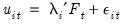
Innovational Outlier Tests
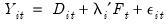
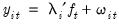
For the IO model, we consider the following general null hypothesis:
 | (42.48) |
where

are
i.i.d. innovations, and
is a lag polynomial representing the dynamics of the stationary and invertible ARMA error process. Note that the break variables enter the model with the same dynamics as the

innovations.
For our alternative hypothesis, we assume a trend stationary model with breaks in the intercept and trend:
 | (42.49) |
with the breaks again following the innovation dynamics.
We may construct a general Dickey-Fuller test equation which nests the two hypotheses:
 | (42.50) |
and use the
t-statistic for comparing
to 1 (
) to evaluate the null hypothesis. As with conventional Dickey-Fuller unit root test equations, the

lagged differences of the

are included in the test equations to eliminate the effect of the error correlation structure on the asymptotic distribution of the statistic.
Within this general framework, we may specify different models for the null and alternative by placing zero restrictions on one or more of the trend and break parameters

,
,
.

. Following Perron (1989), Perron and Vogelsang (1992a, 1992b), and Vogelsang and Perron (1998), we consider four distinct specifications for the Dickey-Fuller regression which correspond to different assumptions for the trend and break behavior:
• Model 0: non-trending data with intercept break:
 | (42.51) |
Setting the trend and trend break coefficients
and

to zero yields a test of a random walk against a stationary model with intercept break.
• Model 1: trending data with intercept break:
 | (42.52) |
Setting the trend break coefficient
to zero produces a test of a random walk with drift against a trend stationary model with intercept break.
• Model 2: trending data with intercept and trend break:
 | (42.53) |
The unrestricted Dickey-Fuller equation tests the random walk with drift against a trend stationary with intercept and trend break alternative.
• Model 3: trending data with trend break:
 | (42.54) |
Setting the intercept break and break dummy coefficients
and
to zero tests a random walk with drift null against a trend stationary with trend break alternative.
Note that the test equation for Model 3 follows the methodology of Zivot and Andrews (1992) and Banerjee
et al. (1992) which does not nest the null and alternatives, as
is absent from the test equation; see Vogelsang and Perron (1998), p. 1077 for discussion.
You should bear in mind that whether one specifies a known break date or estimates the break date from the data affects the allowable specifications for the null hypothesis.
If the break date is known as in Perron (1989), Models 0, 1, and 2 allow for breaks under the null hypothesis. Model 3 does not allow for a break under the null.
If the break date is estimated, the test statistics considered here do not permit a breaking trend under the null. Vogelsang and Perron (1998) offer a detailed discussion of this point, noting that this undesirable restriction is required to obtain distributional results for the resulting Dickey-Fuller
t-statistic. They offer practical advice for testing in the case where you wish to allow

under the null. See also Kim and Perron (2009) for more recent work that directly tackles this issue.
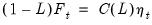
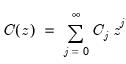
Additive Outlier Tests
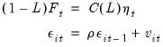
The general AO model null hypothesis is:
 | (42.55) |
where
are
i.i.d. innovations, and
is a lag polynomial representing the dynamics of the stationary and invertible ARMA error process, and
is a drift parameter. Note that the full impact of the break variables occurs immediately.
The alternative hypothesis is for a trend stationary model with possible breaks in the intercept and trend:
 | (42.56) |
Testing for a unit root in the AO framework is a two-step procedure where we first use the intercept, trend, and breaking variables to detrend the series using OLS, and then use the detrended series to test for a unit root using a modified Dickey-Fuller regression.
In the first-step of the AO test, we detrend the data using a model with appropriate trend and break variables:
• Model 0: non-trending data with intercept break:
 | (42.57) |
• Model 1: trending data with intercept break:
 | (42.58) |
• Model 2: trending data with intercept and trend break:
 | (42.59) |
• Model 3: trending data with trend break:
 | (42.60) |
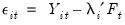
In the second-step, let

be the residuals obtained from the detrending equation. The resulting Dickey-Fuller unit root test equation is given by,
• Models 0, 1, 2:
 | (42.61) |
• Model 3:
 | (42.62) |
where we use the
t-statistic for comparing
to 1,

, to evaluate the null hypothesis.
These are standard augmented Dickey-Fuller equations with the addition of

break dummy variables

in
Equation (42.62) to eliminate the asymptotic dependence of the test statistic on the correlation structure of the errors and to ensure that the asymptotic distribution is identical to that of the corresponding IO specification. See Perron and Vogelsang (1992b) for discussion.
As with the IO tests, when we estimate the break date from the data, the distributional results require that there be no trend break under the null hypothesis. See Vogelsang and Perron (1998) and Kim and Perron (2009) for discussion.
Test Options
For a given test equation described above, you must choose a number of lags
to include in the test equation, and you must specify the candidate date

at which to evaluate the break. EViews offers a number of tools for you to use when making these choices.
Lag Selection
The theoretical properties of the test statistics requires that we choose the number of lag terms in the Dickey-Fuller equations

to be large enough to eliminate the effect of the correlation structure of the errors on the asymptotic distribution of the statistic
• Fixed (with observation-based suggestion from Said and Dickey, 1984).
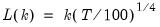
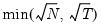
All of the remaining methods are data dependent, and require specification of a maximum lag length

. A different optimal lag length

is obtained for each candidate break date.
• t-test.
Following Perron (1989), Perron and Vogelsang (1992a, 1992b), and Vogelsang and Perron (1998),

is chosen so that the coefficient on the last included dependent variable lag difference is significant at a specified probability value, while the coefficients on the last included lag difference in higher-order autoregressions up to

are all insignificant at the same level. The probability values for the
t-statistics are computed using the
t-distribution.
The t-test method requires the specification of a p-value for use in evaluating significance. The default p-value of 0.10 may be changed by the user.
• F-test.
Based on an approach of Said and Dickey (1984) (see also Perron and Vogelsang, 1992a, 1992b), the approach uses an
F-test of the joint significance of the lag coefficients for a given
against all higher lags up to

. If any of the tests against higher-order lags are significant at a specified probability level, we set

. If none of the test statistics is significant, we lower

by 1 and continue. We begin the procedure with

and continue until we achieve a rejection with

, or until the lower bound

is evaluated without rejection and we set

.
The F-test method requires the specification of a p-value for use in evaluating significance. The default p-value of 0.10 may be changed by the user.
• Information criterion
Following the approach of Hall (1994) and Ng and Perron (1995),

is chosen to minimize the specified information criterion amongst models with 0 to

lags.
You may choose between the Akaike, Schwarz, Hannan-Quinn, Modified Akaike, Modified Schwarz, Modified Hannan-Quinn. Note that the sample used for model selection excludes data using full set of lag differences up to

.
Break Date Selection
Perron (1989) specified an a priori fixed break date. Subsequent research (Zivot and Andrews, 1992; Banerjee et al., 1992; Vogelsang and Perron, 1998) has focused on endogenously determining break dates from the data. EViews supports the following break date selection methods:
• Minimize the Dickey-Fuller
t-statistic

.
Select the date providing the most evidence against the null hypothesis of a unit root and in favor of the breaking trend alternative hypothesis.
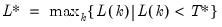
• Minimize or maximize
 t
t-statistic (

) Maximize
 t
t-statistic (

), Minimize or Maximize
 t
t-statistic (

), Maximize
 t
t-statistic (

), Maximize
 F
F-statistic (

).
Choose the date with the strongest evidence of a break. The alternative minimize and maximize options are provided to allow for evaluation of one-sided alternatives, and will produce different critical values for the final Dickey-Fuller test statistic and tests with greater power than the non-directional alternatives.
• User-specified break date.
Specify a fixed break date. This option allows you to carry out the original Perron (1989) test.
For the automatic break selection methods, the following procedure is carried out. For each possible break date, the optimal number of lags

is chosen using the specified method, and the test statistic of interest is computed. The procedure is repeated for each possible break date, and the optimal break date is chosen from the candidate dates.
When the method is minimize

, all possible break dates are considered. For the methods involving

or

, trimming is performed to remove some endpoint values from consideration as the break date.
Computing a Unit Root with Breakpoint Test
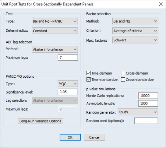
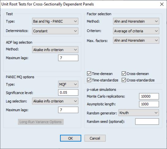
To compute a breakpoint unit root test, open a series window and select to display the dialog:
The dialog is divided into six sections.
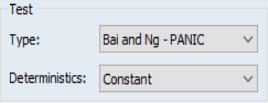
• The first section tells EViews whether you wish to compute the test using the raw data (), or whether to test for higher order integration using differences ( or ) of the original data.
• The section determines the trend components that are included in the test. Using the dropdown, you may choose between an only or an specification. If you include a trend in the specification you will be prompted to indicate which deterministic components are breaking by choosing , , or in the dropdown menu.
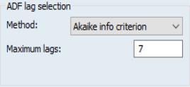
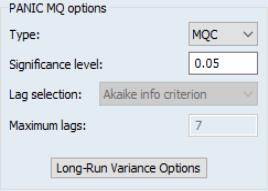
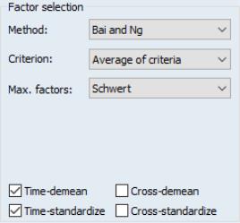
• The section describes the method for selecting lags
for each of the augmented Dickey-Fuller test specifications (
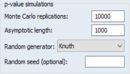
“Lag Selection”). You may choose between (AIC), (BIC), (HQC), , , , , , and lag specifications. For all but the lag method, you must provide a to test; by default, EViews will suggest a maximum lag based on the number of observations in the series. For the test methods (, ), you must specify a
p-value for the tests; for the lag method, you must specify the actual number of use using the edit field.
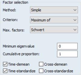
• The section allows you to choose between the default and the specifications (
“The Model”).
For a model with an intercept break, you may choose between minimizing the
t-statistic for

in the ADF test (), minimizing the
t-statistic for the intercept break coefficient (), maximizing the
t-statistic for the break coefficient (), maximizing the absolute value of the
t-statistic for the intercept break coefficient (), or providing a specific date ().
For models with a trend break, there will be corresponding entries for minimizing and maximizing the t-statistic or absolute value of the t-statistic for the trend break coefficient. For models with both an intercept and trend break you will be offered an additional choice of using the F-statistic for the break coefficients () to select the breakpoint.
You will be prompted for specify a trimming percentage when employing methods that involve the t-statistic or F-statistic of the break coefficients, EViews will remove from consideration as the breakpoint this percentage of the observations from each endpoint.
For the break choice you will be prompted to specify a single date.
• Lastly, the controls the output produced by the view. The checkbox controls whether to show only the test results with the selected break, or to show the test results and graphs depicting the break selection criterion results for each candidate break.
If you provide a name in the edit field, EViews will save the results from each of the candidate augmented Dickey-Fuller tests in workfile. The first column contains the observation identifier for the break; the second through fifth columns contain the autoregressive coefficient, autoregressive coefficient standard error, number of observations, number of variables, and number of selected lags in the Dickey-Fuller regressions.
If appropriate, the remaining columns contain results for the breakpoint selection, with the contents varying with the method chosen. When minimizing the Dickey-Fuller

, the output consists of a single column containing the

statistics. For methods involving one of

or

, the output contains the coefficient value, standard error, and the corresponding
t-statistic; for the
F-statistic method, the output columns consist of the estimates of

, the standard error of
, the estimates of

, the standard error of

, and the
F-statistic for testing the significance of the two coefficients.
Examples
As examples, we replicate some of the results given in Perron (1997), using data originally provided by Nelson and Plosser (1982). The dataset contains fourteen annual macroeconomic series with values between 1860 and 1988. These data are provided in the workfile “nelson_plosser.wf1”.
Real GNP
To begin, we replicate the results in the second row of Table 3 in Perron (1997), which tests for a unit root in the log of real GNP using data between 1909 and 1970. We display the log of real GDP, and set the workfile sample to dates from 1909 to 1970 with the commands
smpl 1909 1970
show log(rgnp)
To perform the unit root test with breakpoints, we click on which brings up the test dialog. In this example Perron tests for the existence of a unit root of the data in levels. The test assumes an innovation outlier break, with a trend specification given by Model 2 (
Equation (42.53), above); trending data with both intercept and trend break.
Perron selects a breakpoint by minimizing the Dickey-Fuller t-statistic, and selects a lag length using the F-test.
We can match these settings by clicking the Level and Innovation Outlier buttons, changing the Basic Trend specification to Trend and Intercept and the Breaking Trend specification to Intercept, selecting Dickey-Fuller min-t as the Breakpoint selection, and changing the Lag length Method to F-statistic:
Clicking OK produces the following results:
The top section of this output describes the test that was performed, with a description of the underlying series, the trend and break specification, and the break type. The second section displays the selected break date, which in this case is 1929. Recall that, unlike Perron, EViews reports the break date for the start of the new regime instead of the last date before of the old regime, so the EViews reported date of 1929 matches Perron’s 1928 result. Lastly, we see that the selected number of lags for corresponding test regression, selected on the basis of F-statistic selection is eight.
The lower section reports the Augmented Dickey-Fuller t-statistic for the unit root test, along with Vogelsang’s asymptotic p-values. Our test resulted in a statistic of -5.50, with a p-value less than 0.01, leading us to reject the null hypothesis of a unit root.
EViews also provides a graph of the Augmented Dickey-Fuller statistics and AR coefficients at each test date:
Both graphs show a large dip in 1929, leaving little doubt as to which date should be selected as the break point.
Employment
Our second example replicates row nine of Table 3 in Perron (2007). This example performs a unit root test on the log of employment using data from 1890 to 1970. We again begin with issuing commands to set the sample and display the log of employment:
smpl 1890 1970
show log(totalemp)
In this test, Perron again assumes an innovation outlier break, with a trend specification given by Model 2 (
Equation (42.53), above); trending data with intercept and trend break. However Perron now selects the breakpoint corresponding to the minimum intercept break
t-statistic, and selects the lag-length using the
t-statistic method. We replicate these choices with the following dialog settings:
The first section of the results of this test are shown below:
Again, the top section of this output describes the test that was performed, notably the underlying series, the trend and break specifications, and the break type. From the second section we can see that again a date of 1929 was chosen as the most likely break date. The t-statistic based lag selection selected seven lags for this test regression.
The second section displays the test statistic and associated p-value. The statistic value of -4.918 matches the value report by Perron, and the p-value again means that we reject (at a 5% significance level) the null hypothesis of a unit root.
GNP Deflator
Our final example replicates row 12 of Table 3 in Perron (1997), and performs a unit root test with breaks on the log of the GNP deflator between 1889 and 1970. We set the workfile sample and display the log of the GNP deflator by issuing the commands
smpl 1889 1970
show log(gnpdeflat)
We can mimic Perron’s results with the following dialog settings:
which yield results of:
Here, 1920 was selected at the most likely break date, and the automatic lag selection routine selected 9 lags.
The t-statistic of -3.869 matches that reported by Perron, and the corresponding p-value of 0.27 indicates we cannot reject the hypothesis that the log of the GNP deflator has a unit root.