Examples
Standard ARCH
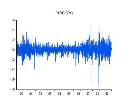
As an illustration of ARCH modeling in EViews, we estimate a model for the daily S&P 500 stock index from 1990 to 1999 (in the workfile “Stocks.WF1”). The dependent variable is the daily continuously compounding return,

, where

is the daily close of the index. A graph of the return series clearly shows volatility clustering.
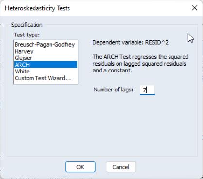
We will specify our mean equation with a simple constant:
For the variance specification, we employ an EGARCH(1, 1) model:
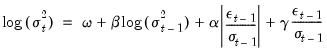 | (27.44) |
When we previously estimated a GARCH(1,1) model with the data, the standardized residual showed evidence of excess kurtosis. To model the thick tail in the residuals, we will assume that the errors follow a Student's t-distribution.
To estimate this model, open the GARCH estimation dialog, enter the mean specification:
dlog(spx) c
select the method, enter 1 for the and orders and the , and select for the . Click on to continue.
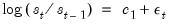
EViews displays the results of the estimation procedure. The top portion contains a description of the estimation specification, including the estimation sample, error distribution assumption, and backcast assumption.
Below the header information are the results for the mean and the variance equations, followed by the results for any distributional parameters. Here, we see that the relatively small degrees of freedom parameter for the t-distribution suggests that the distribution of the standardized errors departs significantly from normality.
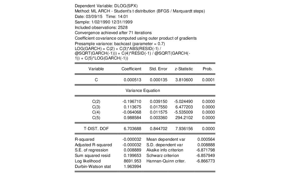
To test whether there any remaining ARCH effects in the residuals, select and specify the order to test. EViews will open the general Heteroskedasticity Tests dialog opened to the ARCH page. Enter “7” in the dialog for the number of lags and click on .
The top portion of the output from testing up-to an ARCH(7) is given by:
so there is little evidence of remaining ARCH effects.
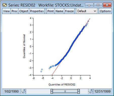
One way of further examining the distribution of the residuals is to plot the quantiles. First, save the standardized residuals by clicking on , select the option, and specify a name for the resulting series. EViews will create a series containing the desired residuals; in this example, we create a series named RESID02. Then open the residual series window and select and from the list of graph types on the left-hand side of the dialog.
If the residuals are normally distributed, the points in the QQ-plots should lie alongside a straight line; see
“Quantile-Quantile (Theoretical)” for details on QQ-plots. The plot indicates that it is primarily large negative shocks that are driving the departure from normality. Note that we have modified the QQ-plot slightly by setting identical axes to facilitate comparison with the diagonal line.
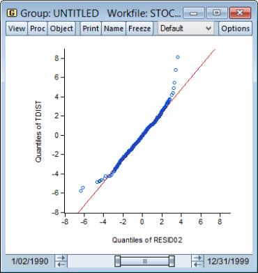
We can also plot the residuals against the quantiles of the t-distribution. Instead of using the built-in QQ-plot for the t-distribution, you could instead simulate a draw from a t-distribution and examine whether the quantiles of the simulated observations match the quantiles of the residuals (this technique is useful for distributions not supported by EViews). The command:
series tdist = @qtdist(rnd, 6.7)
simulates a random draw from the t-distribution with 6.7 degrees of freedom. Then, create a group containing the series RESID02 and TDIST. Select and choose from the left-hand side of the dialog and Empirical from the Q-Q graph dropdown on the right-hand side.
The large negative residuals more closely follow a straight line. On the other hand, one can see a slight deviation from t-distribution for large positive shocks. This is expected, as the previous QQ-plot suggested that, with the exception of the large negative shocks, the residuals were close to normally distributed.
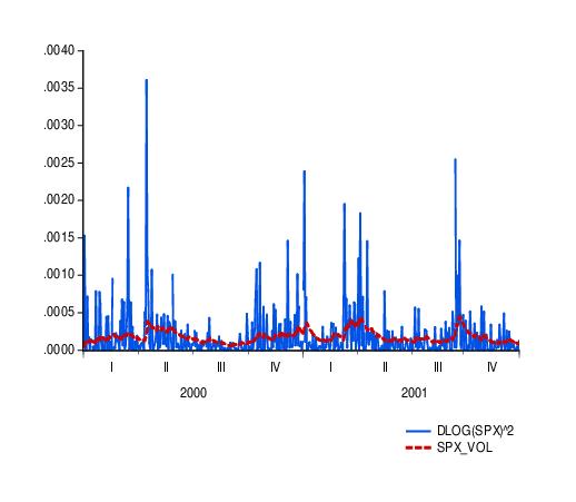
To see how the model might fit real data, we examine static forecasts for out-of-sample data. Click on the button on the equation toolbar, type in “SPX_VOL” in the GARCH field to save the forecasted conditional variance, change the sample to the post-estimation sample period “1/1/2000 1/1/2002” and click on to select a static forecast.
Since the actual volatility is unobserved, we will use the squared return series (DLOG(SPX)^2) as a proxy for the realized volatility. A plot of the proxy against the forecasted volatility for the years 2000 and 2001 provides an indication of the model’s ability to track variations in market volatility.
MIDAS GARCH
The following commands will (as of 2004-04-03) contact the Federal Reserve Data server, fetch the daily SP500 index data (SP500) and the monthly industrial production data (INDPRO) and create new returns series based on the logarithmic changes in those series:
dbopen(type=fred, server=api.stlouisfed.org/fred)
wfcreate(page=daily) d5 2013 @now
fetch sp500
pagecontract if sp500<>na
series returns = dlog(sp500)*100
pagecreate(page=monthly) m 2013 @now
fetch indpro
series d_indpro = dlog(indpro)*100
pageselect daily
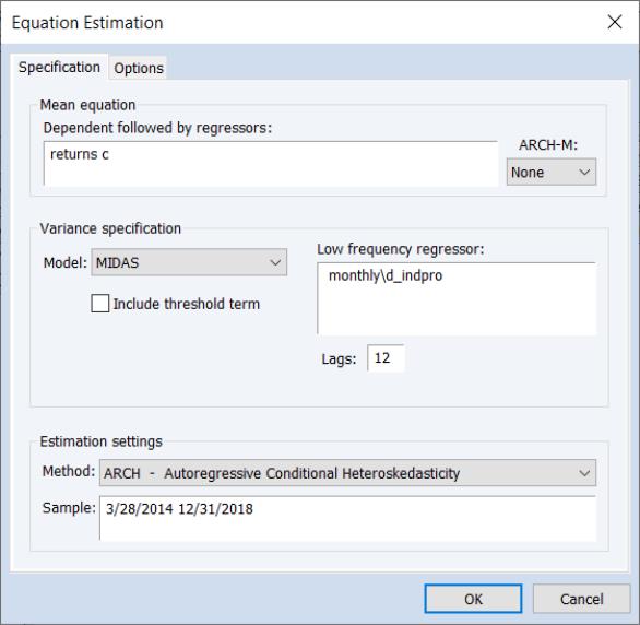
We may then estimate a MIDAS GARCH model for the daily returns, using 12 lags of the monthly industrial production changes as explanatory variables in the permanent component specification.
The MIDAS GARCH dialog may be filled out as follows, with D_INDPRO on the MONTHLY page specified as our low-frequency MIDAS regressor:
and click on to perform the estimation using the remaining default settings.
Alternately, you may issue the following commands to perform the estimation procedure and display results:
smpl @first 2018
equation ex1.arch(midas) returns c @ monthly\d_indpro
show ex1
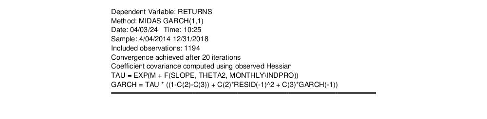
Following estimation, EViews will display the results view. The top portion of the results shows the estimation settings, sample information, computation information, and a brief text description of the transitory and permanent component specifications:
Note that the long-run component TAU is described as the exponential function evaluated at the sum of an intercept term M and a function which depends on a slope coefficient

, the parameter THETA2 (

), and the low frequency series MONTHLY\INDPRO. The variance is described as the product of the long-run component TAU, and the short-run GARCH(1,1) component.
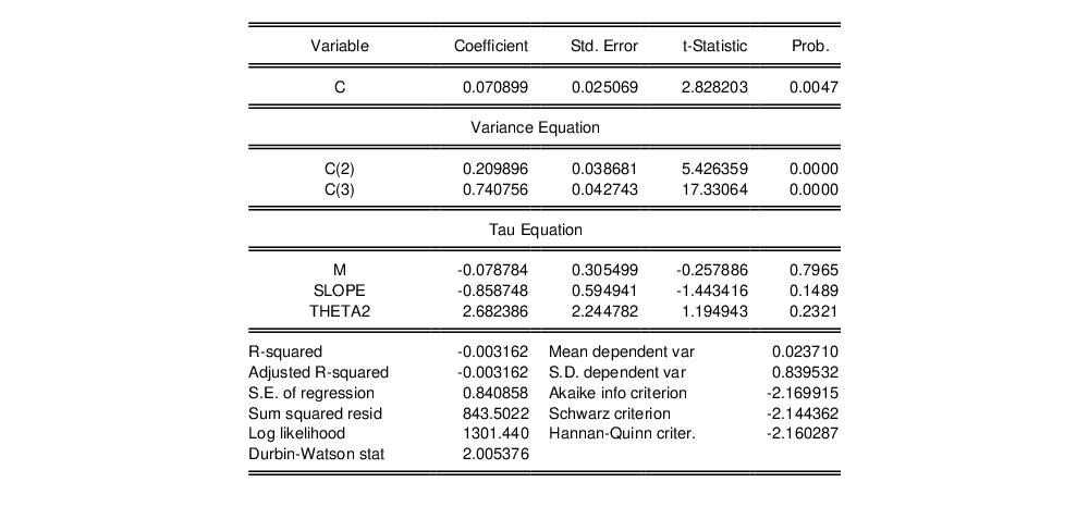
The next section shows standard coefficient results for the mean equation, transitory portion of the variance equation, and the permanent component, as well as summary statistics for the estimated equation:
As is the case with other EViews estimators, you may find it useful to use the view to see the mapping of the results in the output to the underlying coefficients.
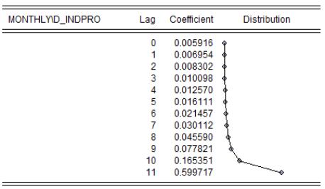
The bottom portion of the results show the distribution of the weight values

for various lags given the estimated

, SLOPE (

), and THETA2 (

):
Following convention, the “Lag 0” coefficient corresponds the

coefficient weight on MONTHLY\D_INDPRO(-1), “Lag 1” corresponds to

and MONTHLY\D_INDPRO(-2), and so forth. The distribution of weights shows that the permanent component in generally increasing in the lags of D_INDPRO, and is most pronounced at D_INDPRO(-12).