Technical Background
For brevity, we will assume the reader has some knowledge of Bayesian statistics, and is familiar with the notions of the prior and posterior distributions and marginal likelihoods.
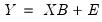
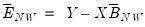
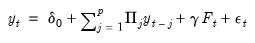
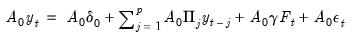
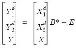
To relate the general Bayesian framework to Vector Autoregressions, we first write the VAR as:
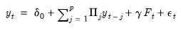 | (47.1) |
where
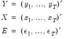
• 
is an

vector of endogenous variables (
i.e. the VAR has

variables and

lags)
• 
is an

vector of intercept coefficients
• 
are

matrices of lag coefficients
• 
is a

vector of exogenous variables
• 
is a

matrix of exogenous coefficients
• 
is an

vector of errors where we assume

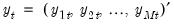
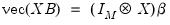
Collecting the right-hand side variables into the

vector

and corresponding coefficients into

,
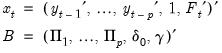 | (47.2) |
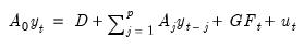
we may rewrite
Equation (47.1) as
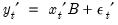 | (47.3) |
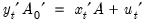
In matrix form, we may stack the observations so we have:
 | (47.4) |
where
 | (47.5) |

and

are

,

is

, and

is

, for

when

presample observations on

are available.
The multivariate normal assumption on the

leads to a multivariate normal distribution for

. Let

and

. Then
and
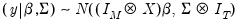 | (47.6) |
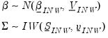
Next, a prior is specified for the model parameters.
Priors
EViews offers seven prior classes which have been popular in the BVAR literature.
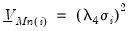
1. The Litterman/Minnesota prior: A normal prior on

with fixed

.
2. The normal-flat prior: A normal prior on

and an improper prior for

.
3. The normal-Wishart prior: A normal prior on

and an inverse Wishart prior on

.
4. The independent normal-Wishart prior. A normal prior on

and an inverse Wishart prior on

.
5. The Sims-Zha normal-flat. A structural VAR equivalent of the normal-flat prior.
6. The Sims-Zha normal-Wishart prior. A structural VAR equivalent of the normal-Wishart prior.
7. The Giannone, Lenza and Primiceri prior. A prior that treats the hyper-parameters as parameters that can be selected through an optimization procedure.
Litterman Prior
Early work on Bayesian VAR priors was done by researchers at the University of Minnesota and the Federal Reserve Bank of Minneapolis (see Litterman (1986) and Doan, Litterman, and Sims (1984)), and these early priors are often referred to as the “Litterman prior” or the “Minnesota prior”.
This family of priors is based on an assumption that

is known; replacing

with an estimate

. This assumption yields simplifications in prior elicitation and computation of the posterior.
Let

. The prior on the

elements of

is assumed to be:
 | (47.7) |
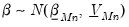
The Litterman prior yields a posterior of:
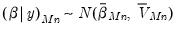 | (47.8) |
where
 | (47.9) |
These posterior distributions are algebraically tractable and only require specification of the prior mean

and covariance

, along with the estimate of

.
The standard implementations of the Litterman prior employ simple formulations for

and

that lead to easy computation of the posterior distributions.
First,

is set to a vector of nearly all zeros, with only the elements corresponding to a variable’s own first lag being non-zero. Those own lag elements are generally set to 1 or 0, as specified by the hyper-parameter

.
Second,

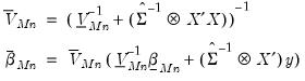
is assumed to be a diagonal matrix:
• The diagonal elements corresponding to the
j-th endogenous variables in the
i-th equation at lag

are given by:
 | (47.10) |
• The diagonal elements corresponding to all of the exogenous variables (including the constant) in the

-th equation are:
 | (47.11) |

,

,

, and

are hyper-parameters, and

is the square root of the corresponding diagonal element of

.
Normal-Flat Prior
The normal-flat relaxes the assumption of

being known but imposes an improper prior on

.
For

, the prior is from a normal distribution conditional on

:
 | (47.12) |
For

, all of the prior information is contained in the degrees-of-freedom parameter

.
The conditional posterior of

is also from a normal distribution:
 | (47.13) |
where
 | (47.14) |
The posterior of

is inverse-Wishart:
 | (47.15) |
where

denotes the inverse-Wishart distribution.
The conditional posteriors only require specification of

,

, and

.

is constructed identically to the Litterman prior as a vector of nearly all zeros, with only the elements corresponding to an endogenous variable’s own first lag, optionally set to a non-zero value specified by the hyper-parameter

.
The remaining hyper-parameters are constructed as:
 | (47.16) |
Where

and

are scalars.
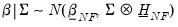
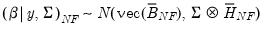
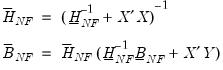
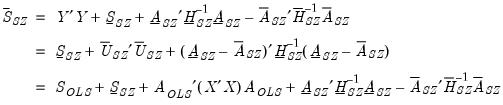
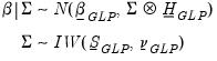
Normal-Wishart Prior
The normal-Wishart prior again relaxes the assumption of

being known, this time imposing a prior distribution.
For the normal-Wishart model, the priors for alpha and Sigma are given by:
 | (47.17) |
The conditional posterior for

is
 | (47.18) |
and the posterior of

is,
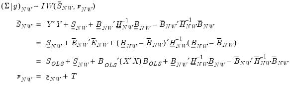 | (47.19) |
where

and

are estimates from a conventional VAR, and
. Note the three calculations of

are algebraically equivalent, and all three appear in the literature.
Again, these posterior distributions and likelihood are algebraically tractable and only require specification of

and

, along with prior specifications of

and

.

is constructed identically to the Litterman prior as a vector of nearly all zeros, with only the elements corresponding to an endogenous variable’s own first lag, optionally set to a non-zero value specified by the hyper-parameter

.
The remaining hyper-parameters are constructed as:
 | (47.20) |
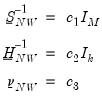
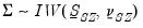
Independent Normal-Wishart Prior
The independent normal-Wishart prior is similar to the normal-Wishart prior, but allows cross-equation independence of the coefficient distributions and removes the dependence of

on

.
It is worth noting that the independent normal-Wishart prior typically referenced in the literature (notably, Koop and Korobilis 2009) also allows for differing variables in each endogenous variable’s equation (restricted VARs). EViews currently does not allow for restricted VARs under this prior.
The independent normal-Wishart priors for

and

are:
 | (47.21) |
where
,

is

, and

is

. Note the cross-equation independence of the prior implies that

is of full size.
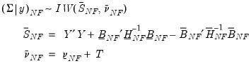
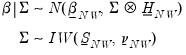
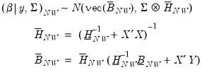
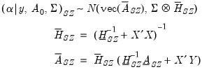
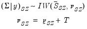
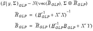
The unconditional posterior distributions from these priors are non-tractable. However, conditional posterior distributions are:
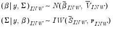 | (47.22) |
where
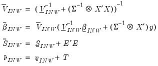 | (47.23) |
These conditional posteriors can be used in a Gibbs sampler to obtain properties of the unconditional posterior. Draws are taken sequentially from the conditional distributions (starting with an initial value for

to draw

), then, after discarding a number of burn-in draws, taking the mean of the draws.
The marginal likelihood also does not have an analytical solution, but an estimate of its value can be computed from the outputs of the Gibbs sampler using Chib’s method (1995).
The prior hyper-parameters are constructed in a similar manner to the normal-Wishart prior;

is a vector of nearly all zeros, with only the elements corresponding to a variable’s own first lag, the hyper-parameter

, optionally set to non-zero values.
The remaining hyper-parameters are constructed as:
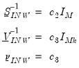 | (47.24) |
where

,

, and

are scalars.
Sims-Zha Priors
Sims-Zha (1998), is one of the earliest expansions of the Litterman prior to allow for an unknown

.
(Note that the Sims-Zha approach simultaneously uses dummy observations to account for unit-root and cointegration issues (
“Dummy Observations”), alongside a specific Bayesian prior form. We have separated these two concepts to allow dummy observations to be used with any prior, however it should be noted that researchers referring to the “Sims-Zha” priors generally imply use of both their prior and the inclusion of dummy observations.)
The construction of their prior employs the structural form of the VAR. To begin recall the standard reduced form VAR representation:
 | (47.25) |
It follows that
 | (47.26) |
or
 | (47.27) |
which is the structural representation of the VAR. We may write this equation as:
 | (47.28) |
where
 | (47.29) |
and we assume with
.
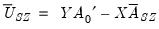
In matrix form, we may stack the observations so we have:
 | (47.30) |

and

are defined as before,

is

,

is

, and

is

, for
when

presample observations on

are available.
Sims-Zha place a conditional prior on

given

, using either the normal-flat or normal-Wishart distributions.
For both distributions, the conditional prior of

is given by:
 | (47.31) |
For the normal-Wishart, the prior on

is:
 | (47.32) |
where

is

The resulting conditional posterior for

is then:
 | (47.33) |
And the posterior for

is:
 | (47.34) |
where, for the normal-flat prior,
 | (47.35) |
and for the normal-Wishart prior,
 | (47.36) |
where

and

are estimates obtained from a conventional VAR, and
.
The expressions for the posterior distribution do not require specification of a prior on

. However, formulation of the marginal likelihood does require a prior on

, and as such, EViews does not report a marginal likelihood.
Sims-Zha suggest a form of

and

along similar lines to the Litterman priors.
First,

is set to a vector of nearly all zeros, with only the elements corresponding to a variable’s own first lag, hyper-parameter

, being non-zero.
Second

is assumed to be diagonal:
• The diagonal elements corresponding to the
j-th endogenous variables in the
i-th equation at lag

are given by:
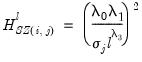 | (47.37) |
• The diagonal elements corresponding to the constants are:
 | (47.38) |
• The diagonal elements corresponding to the remaining exogenous are:
 | (47.39) |

,

,

,

and

are hyper-parameters, and

is the square root of the corresponding diagonal element of

.
Note that the Sims-Zha prior treats the elements of the covariance prior slightly differently from the Litterman prior—there is no cross-variable relative weight term,

, and there are different weights for the constant compared with other exogenous variables.
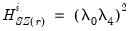
Giannone, Lenza and Primiceri (GLP) Prior
The Giannone, Lenza and Primiceri (GLP) approach constructs the prior in a different manner than the previously outlined methods. GLP begins with a normal-Wishart prior where the specification of the coefficient covariance is akin to a modified Litterman approach. They note that since the marginal likelihood can be derived analytically, and the likelihood is a function of the hyper-parameters, rather than specifying exact values for those parameters, and optimization algorithm can be used to find the optimal specification of the prior.
The prior takes the form:
 | (47.40) |
where
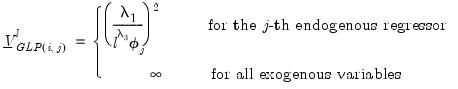 | (47.41) |

is again all zero other than for an endogenous variable’s own first lag.

is diagonal, with each of the diagonal elements a hyper-parameter that is either fixed at an initial covariance matrix or optimized.

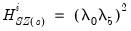
is a pre-specified scalar hyper-parameter:
 | (47.42) |
The conditional posterior for

is then:
 | (47.43) |
And the posterior for

is:
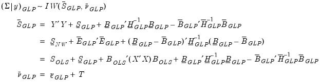 | (47.44) |
where
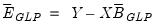
.
This marginal likelihood is maximized with respect to the hyper-parameters to find the optimal parameter values.
Dummy Observations
Sims-Zha (1998) also popularized the idea of complimenting the prior by adding dummy observations to the data matrices in order to improve the forecasting performance of the Bayesian VAR. These dummy observations are made up of two components; the sum-of-coefficient component and the dummy-initial-observation component. Both sets of observations can be applied to any of the above priors.
Sum-of-coefficient
The sum-of-coefficient component of a prior was introduced by Doan, Litterman and Sims (1984) and demonstrates the belief that the average of lagged values of a variable can act as a good forecast of that variable. It also expresses that knowing the average of lagged values of a second variable does not improve the forecast of the first variable.
The prior is constructed by adding additional observations at the top (pre-sample) of the data matrices. Specifically, the following observations are constructed:
 | (47.45) |
where

is the mean of the
i-th variable over the first

-th periods.
These observations introduce correlation between each variable in each equation.

is a hyper-parameter. If

, the observations are uninformative. As

, the observations imply unit roots in each equation, ruling out cointegration.
Dummy- initial-observation
The dummy-initial-observation component (Sims, 1993) creates a single dummy observation which is equal to the scaled average of initial conditions, and reflects the belief that the average of initial values of a variable is likely to be a good forecast of that variable. The observation is formed as:
 | (47.46) |
The hyper-parameter

, is a scaling factor. If

, the observation is uninformative. As

, all endogenous variables in the VAR are set to their unconditional mean, the VAR exhibits unit roots without drift, and the observation is consistent with cointegration.
Augmented Data
The dummy observations are stacked on top of each other, and on top of the original data matrices:
 | (47.47) |
It should be noted that the dummy observations require a correction to the marginal likelihood calculations for each prior.
A Note on Initial Residual Covariance Calculation
Most of the prior types allowed by EViews require an initial value for the residual covariance matrix,

, as an input.
For the Litterman prior,

is taken as known. Since it is not known in practice, an estimate is used in the construction of the prior covariance for

,

. For the independent normal Wishart prior, the initial covariance matrix is used as the starting point for the Gibbs sampler.
Both Sims-Zha priors use the initial covariance to form the prior covariance for

. The Giannone, Lenza and Primiceri prior uses the initial

to form the prior covariance matrix, either as a fixed element, or as the starting point for the optimization routine.
There is no standard method in the literature for selecting the initial covariance matrix.
Researchers wishing to replicate existing studies should pay careful attention to the initial covariance calculation method. The wide variety of options offered by EViews should cover most cases.
 and
and  is
is  .
. and
and  is
is  .
. ,
,  is
is  , and
, and  is
is  .
. ,
,  and
and  are scalars.
 and
and  is
is  .
.