Estimating BTVCVAR in EViews
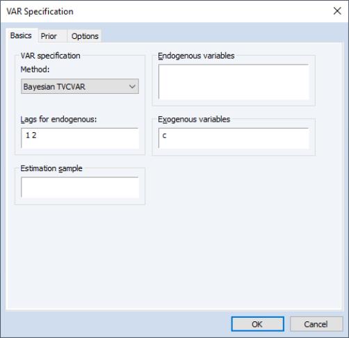
To estimate BTVCVAR in EViews, click on or run var in the command window. EViews will open the dialog. Select from the dropdown menu to display the TVCVAR dialog:
The dialog has three distinct tabs (, , and ).
The endogenous variables, lag specification, exogenous variables, and the estimation sample are set in the tab. The lags are required to be contiguous.
EViews gives users the option of setting aside a subset of the estimation sample for the purpose of specifying a prior distribution. The observations that go towards specifying the prior comprise the prior sample. The remaining observations make up the data sample, which is used to update the prior. See
“Prior Specification” for details.
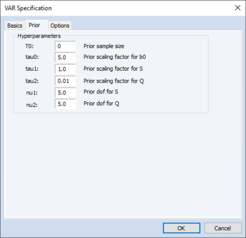
Prior hyper-parameters are set inside the tab. To help with setting the prior, EViews maps the BTVCVAR prior hyper-parameters to a set of six scalar quantities. Users set these scalars to specify a prior sample, control the variability of the time-varying coefficients, etc. See the
“Prior Specification” for details.
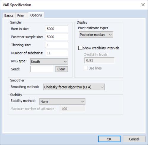
There are four categories in the tab: , , , and .
The options determine how the posterior sample is generated.
• The is the number of initial draws to discard. It is specified as a count. The burn-in process gives the underlying Markov chain time to converge to the posterior distribution.
• The is used to determine how many posterior draws are used to carry out post-updating procedures (estimation, forecasting, impulses responses analysis, etc.).
• The is used to thin the Markov chain. A thinning size of

indicates that every

-th draw is stored. For example, no thinning occurs when

is set to 1, and every other draw is stored when

is set to 2. By definition, thinning does not apply to burn-in draws.
• The field determines how many subchains are used when the posterior sample gets regenerated. Regeneration is typically much faster than initial generation since subchains can be run in parallel.
• The and field is used to set the random number generator and the random seed for the posterior simulator. EViews will generate a seed automatically if the user does not specify one. Click to clear the seed field.
options determine what to report as estimation results. Users can pick either posterior median or posterior mean as their point estimate. The point estimate type selected here will be applied to the coefficients, the observation covariance matrix, and the errors. Users can also display equal-tailed credibility intervals (bands) at one or more credibility levels for the coefficients. To do so, check the box next to . Bands use shading by default. To use lines instead, check the box next to .
A simulation smoother can be selected from the dropdown menu under . EViews currently supports three simulation smoothers: the (CFA), the (KFS), and the method of (MMP). For more information, see McCausland, Miller, & Pelletier (2011) and the references therein.
To enforce stable VAR coefficients at each date within the data sample, select from the dropdown menu under . The threshold ensures that the sampler does not get stuck in an infinite loop in an attempt to obtain stable draws.
Once the BTVCVAR model has been specified, click on to run the posterior simulator. Progress is displayed in the bottom left corner of the EViews window. Once posterior simulation is complete, estimates and other statistics based on the posterior sample are computed.
Estimation results are presented in a spool-like object. The nodes under in the left pane are used for navigation. For example, clicking on the node will bring the summary table into focus. The checkboxes that appear below are used to show/hide coefficient series that are associated to specific endogenous variables, lags, and exogenous variables. For example, unchecking the box next to hides the coefficient series associated to the constant term in all graphs.