Implementation Details
Prior Specification
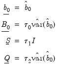
The prior hyper-parameters are

,

,

,

,

, and

. Users set prior hyper-parameters through the six scalar quantities

,

,

,

,

, and

.

is the prior sample size,

is a scaling factor controlling the prior variance of

,

and

are prior scaling factors for

and

, respectively, and

and

are prior degrees of freedom parameters.
Users have the option to set aside the first

observations of the estimation sample for the purpose of specifying the prior distribution. The way in which the scalar quantities map to the original prior hyper-parameters depends on whether a prior sample is present.
Let

and

denote OLS results based on the prior sample. If

, where

is the number of coefficients per equation, then the mapping
is used. When a prior sample is not present, i.e., when

, then the mapping is given by
 | (48.5) |
Entering invalid values for

(e.g.,

) returns an error.
Posterior Simulation
Posterior simulation is carried out using the Gibbs sampler, which is a Markov chain Monte Carlo (MCMC) method for sampling from multivariate densities. It generates a Markov chain by iteratively sampling from the full conditionals of the target density. Draws obtained after the burn-in period are used to compute estimates, generate predictions, and so on.
The chain is initialized at the mode of the prior. Posterior full conditionals are described below.
Posterior Full Conditional for b
Let
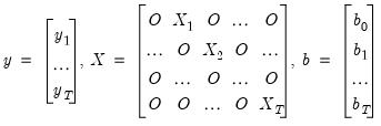 | (48.6) |
where the  's are zero matrices. Let
 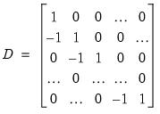 | (48.7) |
denote the square  matrix of first differences. Then
 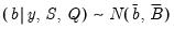 | (48.8) |
where
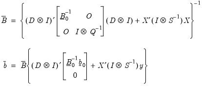 | (48.9) |
Posterior Full Conditional for S
Let
denote the matrix of observation errors. Then
where
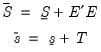 | (48.10) |
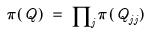
Posterior Full Conditional for Q
Let
denote the matrix of process errors. Then
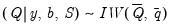 | (48.11) |
where
 | (48.12) |
Diagonal Q
EViews follows the common practice of requiring

to be diagonal. Under this restriction, the prior on

cannot be inverse Wishart. Instead, we have
where the prior on the

-th diagonal element

is given by
The notation

and

are as they were defined in the unrestricted case. It can be shown that the posterior full conditional for

is
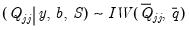 | (48.13) |
where

and

are as they were defined in the unrestricted case. Conditioning on other diagonal elements is suppressed in the notation; notice that the diagonal elements of

are conditionally independent in any case.
Memory Use
Following posterior simulation, a BTVCVAR object will hold onto draws until either the object is deleted or the workfile is closed. Estimation results are written to disk; therefore, a BTVCVAR object in a saved workfile can display estimation results without having to regenerate the posterior sample. Regeneration of the posterior sample is required if display options are changed or when conducting other post-sampling procedures.
Replications
For reproducibility, set the random seed, the random number generator type, and the number of subchains to override the default values.
When a posterior sample is regenerated, it has the same set of draws as the original sample. If the posterior sample cannot be regenerated for any reason, EViews will give you the option to generate a new set of draws.