Background
We begin with a brief sketch of the basic features of the common factor model. Our notation parallels the discussion in Johnston and Wichtern (1992).
The Model
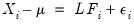
The factor model assumes that for individual

, the
observable multivariate

-vector

is generated by:
 | (60.1) |
where

is a

vector of variable means,

is a

matrix of coefficients,

is a

vector of standardized
unobserved variables, termed
common factors, and

is a

vector of errors or
unique factors.
The model expresses the

observable variables

in terms of

unobservable common factors

, and

unobservable unique factors

. Note that the number of unobservables exceeds the number of observables.
The
factor loading or
pattern matrix

links the unobserved common factors to the observed data. The
j-th row of

represents the loadings of the
j-th variable on the common factors. Alternately, we may view the row as the coefficients for the common factors for the
j-th variable.
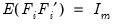
To proceed, we must impose additional restrictions on the model. We begin by imposing moment and covariance restrictions so that

and

,

,
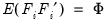
, and

where

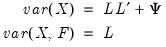
is a diagonal matrix of unique variances. Given these assumptions, we may derive the fundamental variance relationship of factor analysis by noting that the variance matrix of the observed variables is given by:
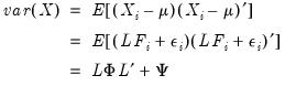 | (60.2) |
The variances of the individual variables may be decomposed into:
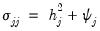 | (60.3) |
for each

, where the

are taken from the diagonal elements of

, and

is the corresponding diagonal element of

.

represents common portion of the variance of the
j-th variable, termed the
communality, while

is the unique portion of the variance, also referred to as the
uniqueness.
Furthermore, the factor structure matrix containing the correlations between the variables and factors may be obtained from:
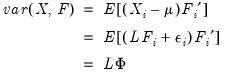 | (60.4) |
Initially, we make the further assumption that the factors are orthogonal so that

(we will relax this assumption shortly). Then:
 | (60.5) |
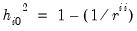
Note that with orthogonal factors, the communalities

are given by the diagonal elements of

(the row-norms of

).
The primary task of factor analysis is to model the

observed variances and covariances of the

as functions of the

factor loadings in

, and

specific variances in

. Given estimates of

and

, we may form estimates of the fitted
total variance matrix,
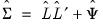
, and the fitted
common variance matrix,

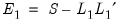
. If

is the observed dispersion matrix, we may use these estimates to define the
total variance residual matrix

and the common variance residual
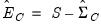
.
Number of Factors
Choosing the number of factors is generally agreed to be one of the most important decisions one makes in factor analysis (Preacher and MacCallum, 2003; Fabrigar, et al., 1999; Jackson, 1993; Zwick and Velicer, 1986). Accordingly, there is a large and varied literature describing methods for determining the number of factors, of which the references listed here are only a small subset.
Kaiser-Guttman, Minimum Eigenvalue
The Kaiser-Guttman rule, commonly termed “eigenvalues greater than 1,” is by far the most commonly used method. In this approach, one computes the eigenvalues of the unreduced dispersion matrix, and retains as many factors as the number eigenvalues that exceed the average (for a correlation matrix, the average eigenvalue is 1, hence the commonly employed description). The criterion has been sharply criticized by many on a number of grounds (e.g., Preacher and MacCallum, 2003), but remains popular.
Fraction of Total Variance
The eigenvalues of the unreduced matrix may be used in a slightly different fashion. You may choose to retain as many factors are required for the sum of the first

eigenvalues to exceed some threshold fraction of the total variance. This method is used more often in principal components analysis where researchers typically include components comprising 95% of the total variance (Jackson, 1993).
Minimum Average Partial
Velicer’s (1976) minimum average partial (MAP) method computes the average of the squared partial correlations after

components have been partialed out (for
). The number of factor retained is the number that minimizes this average. The intuition here is that the average squared partial correlation is minimized where the residual matrix is closest to being the identity matrix.
Zwick and Velicer (1986) provide evidence that the MAP method outperforms a number of other methods under a variety of conditions.
Broken Stick
We may compare the relative proportions of the total variance that are accounted for by each eigenvalue to the expected proportions obtained by chance (Jackson, 1993). More precisely, the broken stick method compares the proportion of variance given by j-th largest eigenvalue of the unreduced matrix with the corresponding expected value obtained from the broken stick distribution. The number of factors retained is the number of proportions that exceed their expected values.
Standard Error Scree
The Standard Error Scree (Zoski and Jurs, 1996) is an attempt to formalize the visual comparisons of slopes used in the visual scree test. It is based on the standard errors of sets of regression lines fit to later eigenvalues; when the standard error of the regression through the later eigenvalues falls below the specified threshold, the remaining factors are assumed to be negligible.
Parallel Analysis
Parallel analysis (Horn, 1965; Humphreys and Ilgen, 1969; Humphreys and Montanelli, 1975) involves comparing eigenvalues of the (unreduced or reduced) dispersion matrix to results obtained from simulation using uncorrelated data.
The parallel analysis simulation is conducted by generating multiple random data sets of independent random variables with the same variances and number of observations as the original data. The Pearson covariance or correlation matrix of the simulated data is computed and an eigenvalue decomposition performed for each data set. The number of factors retained is then based on the number of eigenvalues that exceed their simulated counterpart. The threshold for comparison is typically chosen to be the mean values of the simulated data as in Horn (1965), or a specific quantile as recommended by Glorfeld (1995).
Bai and Ng
Bai and Ng (2002) propose a model selection approach to determining the number of factors in a principal components framework. The technique involves least squares regression using different numbers of eigenvalues obtained from a principal components decomposition. See
“Bai and Ng” for details.
Ahn and Horenstein
Ahn and Horenstein (AH, 2013) provide a method for obtaining the number of factors that exploits the fact that the

largest eigenvalues of a given matrix grow without bounds as the rank of the matrix increases, whereas the other eigenvalues remain bounded. The optimization strategy is then simply to find the maximum of the ratio of two adjacent eigenvalues. See
“Ahn and Horenstein” for discussion.
Estimation Methods
There are several methods for extracting (estimating) the factor loadings and specific variances from an observed dispersion matrix.
EViews supports estimation using maximum likelihood (ML), generalized least squares (GLS), unweighted least squares (ULS), principal factors and iterated principal factors, and partitioned covariance matrix estimation (PACE).
Minimum Discrepancy (ML, GLS, ULS)
One class of extraction methods involves minimizing a discrepancy function with respect to the loadings and unique variances (Jöreskog, 1977). Let

represent the observed dispersion matrix and let the fitted matrix be
. Then the discrepancy functions for ML, GLS, and ULS are given by:
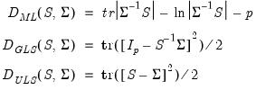 | (60.6) |
Each estimation method involves minimizing the appropriate discrepancy function with respect to the loadings matrix

and unique variances

. An iterative algorithm for this optimization is detailed in Jöreskog. The functions all achieve an absolute minimum value of 0 when

, but in general this minimum will not be achieved.
The ML and GLS methods are scale invariant so that rescaling of the original data matrix or the dispersion matrix does not alter the basic results. The ML and GLS methods do require that the dispersion matrix be positive definite.
ULS does not require a positive definite dispersion matrix. The solution is equivalent to the iterated principal factor solution.
Principal Factors
The principal factor (principal axis) method is derived from the notion that the common factors should explain the common portion of the variance: the off-diagonal elements of the dispersion matrix and the communality portions of the diagonal elements. Accordingly, for some initial estimate of the unique variances

, we may define the reduced dispersion matrix
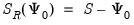
, and then fit this matrix using common factors (see, for example, Gorsuch, 1993).
The principal factor method fits the reduced matrix using the first

eigenvalues and eigenvectors. Loading estimates,

are be obtained from the eigenvectors of the reduced matrix. Given the loading estimates, we may form a common variance residual matrix,
. Estimates of the uniquenesses are obtained from the diagonal elements of this residual matrix.
Communality Estimation
The construction of the reduced matrix is often described as replacing the diagonal elements of the dispersion matrix with estimates of the communalities. The estimation of these communalities has received considerable attention in the literature. Among the approaches are (Gorsuch, 1993):
• Fraction of the diagonals: use a constant fraction

of the original diagonal elements of

. One important special case is to use

; the resulting estimates may be viewed as those from a truncated principal components solution.
• Largest correlation: select the largest absolution correlation of each variable with any other variable in the matrix.
• Squared multiple correlations (SMC): by far the most popular method; uses the squared multiple correlation between a variable and the other variables as an estimate of the communality. SMCs provide a conservative communality estimate since they are a lower bound to the communality in the population. The SMC based communalities are computed as
, where

is the
i-th diagonal element of the inverse of the observed dispersion matrix. Where the inverse cannot be computed we may employ instead the generalized inverse.
Iteration
Having obtained principal factor estimates based on initial estimates of the communalities, we may repeat the principal factors extraction using the row norms of

as updated estimates of the communalities. This step may be repeated for a fixed number of iterations, or until the results are stable.
While the approach is a popular one, some authors are strongly opposed to iterating principal factors to convergence (e.g., Gorsuch, 1983, p. 107–108). Performing a small number of iterations appears to be less contentious.
Partitioned Covariance (PACE)
Ihara and Kano (1986) provide a closed-form (non-iterative) estimator for the common factor model that is consistent, asymptotically normal, and scale invariant. The method requires a partitioning of the dispersion matrix into sets of variables, leading Cudeck (1991) to term this the partitioned covariance matrix estimator (PACE).
Different partitionings of the variables may lead to different estimates. Cudeck (1991) and Kano (1990) independently propose an efficient method for determining a desirable partioning.
Since the PACE estimator is non-iterative, it is especially well suited for estimation of large factor models, or for providing initial estimates for iterative estimation methods.
Model Evaluation
One important step in factor analysis is evaluation of the fit of the estimated model. Since a factor analysis model is necessarily an approximation, we would like to examine how well a specified model fits the data, taking account the number of parameters (factors) employed and the sample size.
There are two general classes of indices for model selection and evaluation in factor analytic models. The first class, which may be termed absolute fit indices, are evaluated using the results of the estimated specification. Various criteria have been used for measuring absolute fit, including the familiar chi-square test of model adequacy. There is no reference specification against which the model is compared, though there may be a comparison with the observed dispersion of the saturated model.
The second class, which may be termed relative fit indices, compare the estimated specification against results for a reference specification, typically the zero common factor (independence model).
Before describing the various indices we first define the chi-square test statistic as a function of the discrepancy function,
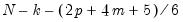
, and note that a model with

variables and

factors has
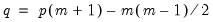
free parameters (

factor loadings and

uniqueness elements, less

implicit zero correlation restrictions on the factors). Since there are

distinct elements of the dispersion matrix, there are a total of
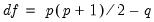
remaining degrees-of-freedom.
One useful measure of the parsimony of a factor model is the parsimony ratio:
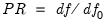
, where

is the degrees of freedom for the independence model.
Note also that the measures described below are not reported for all estimation methods.
Absolute Fit
Most of the absolute fit measures are based on number of observations and conditioning variables, the estimated discrepancy function,

, and the number of degrees-of-freedom.
Discrepancy and Chi-Square Tests
The discrepancy functions for ML, GLS, and ULS are given by
Equation (60.6). Principal factor and iterated principal factor discrepancies are computed using the ULS function, but will generally exceed the ULS minimum value of

.
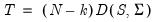
Under the multivariate normal distributional assumptions and a correctly specified factor specification estimated by ML or GLS, the chi-square test statistic

is distributed as an asymptotic

random variable with

degrees-of-freedom (
e.g., Hu and Bentler, 1995). A large value of the statistic relative to the

indicates that the model fits the data poorly (appreciably worse than the saturated model).
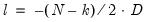
It is well known that the performance of the

statistic is poor for small samples and non-normal settings. One popular adjustment for small sample size involves applying a Bartlett correction to the test statistic so that the multiplicative factor

in the definition of

is replaced by
(Johnston and Wichern, 1992).
Note that two distinct sets of chi-square tests that are commonly performed. The first set compares the fit of the estimated model against a saturated model; the second set of tests examines the fit of the independence model. The former are sometimes termed tests of model adequacy since they evaluate whether the estimated model adequately fits the data. The latter tests are sometimes referred to as test of sphericity since they test the assumption that there are no common factors in the data.
Information Criteria
Standard information criteria (IC) such as Akaike (AIC), Schwarz (SC), Hannan-Quinn (HQ) may be adapted for use with ML and GLS factor analysis. These indices are useful measures of fit since they reward parsimony by penalizing based on the number of parameters.
Construction of the EViews factor analysis information criteria measure employ a scaled version of the discrepancy as the log-likelihood,
, and begins by forming the standard IC. Following Akaike (1987), we re-center the criteria by subtracting off the value for the saturated model, and following Cudeck and Browne (1983) and EViews convention, we further scale by the number of observations to eliminate the effect of sample size. The resulting factor analysis form of the information criteria are given by:
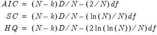 | (60.7) |
You should be aware that these statistics are often quoted in unscaled form, sometimes without adjusting for the saturated model. Most often, if there are discrepancies, multiplying the EViews reported values by

will line up results. Note also that the current definition uses the adjusted number of observations in the numerator of the leading term.
When using information criteria for model selection, bear in mind that the model with the smallest value is considered most desirable.
Other Measures
The root mean square residual (RMSR) is given by the square root of the mean of the unique squared total covariance residuals. The standardized root mean square residual (SRMSR) is a variance standardized version of this RMSR that scales the residuals using the diagonals of the original dispersion matrix, then computes the RMSR of the scaled residuals (Hu and Bentler, 1999).
There are a number of other measures of absolute fit. We refer you to Hu and Bentler (1995, 1999) and Browne and Cudeck (1993), McDonald and Marsh (1990), Marsh, Balla and McDonald (1988) for details on these measures and recommendations on their use. Note that where there are small differences in the various descriptions of the measures due to degree-of-freedom corrections, we have used the formulae provided by Hu and Bentler (1999).
Incremental Fit
Incremental fit indices measure the improvement in fit of the model over a more restricted specification. Typically, the restricted specification is chosen to be the zero factor or independence model.
EViews reports up to five relative fit measures: the generalized Tucker-Lewis Nonnormed Fit Index (NNFI), Bentler and Bonnet’s Normed Fit Index (NFI), Bollen’s Relative Fit Index (RFI), Bollen’s Incremental Fit Index (IFI), and Bentler’s Comparative Fit Index (CFI). See Hu and Bentler (1995)for details.
Traditionally, the rule of thumb was for acceptable models to have fit indices that exceed 0.90, but recent evidence suggests that this cutoff criterion may be inadequate. Hu and Bentler (1999) provide some guidelines for evaluating values of the indices; for ML estimation, they recommend use of two indices, with cutoff values close to 0.95 for the NNFI, RFI, IFI, CFI.
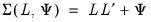
Rotation
The estimated loadings and factors are not unique; we may obtain others that fit the observed covariance structure identically. This observation lies behind the notion of factor rotation, in which we apply transformation matrices to the original factors and loadings in the hope of obtaining a simpler factor structure.
To elaborate, we begin with the orthogonal factor model from above:
 | (60.8) |
where
. Suppose that we pre-multiply our factors by a

rotation matrix

where

. Then we may re-write the factor model
Equation (60.1) as:
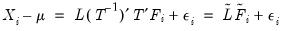 | (60.9) |
which is an observationally equivalent common factor model with rotated loadings
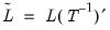
and factors

, where the correlation of the rotated factors is given by:
 | (60.10) |
See Browne (2001) and Bernaards and Jennrich (2005) for details.
Types of Rotation
There are two basic types of rotation that involve different restrictions on

. In
orthogonal rotation, we impose

constraints on the transformation matrix

so that

, implying that the rotated factors are orthogonal. In
oblique rotation, we impose only

constraints on

, requiring the diagonal elements of

equal 1.
There are a large number of rotation methods. The majority of methods involving minimizing an objective function that measure the complexity of the rotated factor matrix with respect to the choice of

, subject to any constraints on the factor correlation. Jennrich (2001, 2002) describes algorithms for performing orthogonal and oblique rotations by minimizing complexity objective.
For example, suppose we form the

matrix

where every element

equals the square of a corresponding factor loading

:

. Intuitively, one or more measures of simplicity of the rotated factor pattern can be expressed as a function of these squared loadings. One such function defines the Crawford-Ferguson family of complexities:
 | (60.11) |
for weighting parameter

. The Crawford-Ferguson (CF) family is notable since it encompasses a large number of popular rotation methods (including Varimax, Quartimax, Equamax, Parsimax, and Factor Parsimony).
The first summation term in parentheses, which is based on the outer-product of the
i-th row of the squared loadings, provides a measure of complexity. Those rows which have few non-zero elements will have low complexity compared to rows with many non-zero elements. Thus, the first term in the function is a measure of the row (variables) complexity of the loadings matrix. Similarly, the second summation term in parentheses is a measure of the complexity of the
j-th column of the squared loadings matrix. The second term provides a measure of the column (factor) complexity of the loadings matrix. It follows that higher values for

assign greater weight to factor complexity and less weight to variable complexity.
Along with the CF family, EViews supports the following rotation methods:
| | |
Biquartimax | • | • |
Crawford-Ferguson | • | • |
Entropy | • | |
Entropy Ratio | • | |
Equamax | • | • |
Factor Parsimony | • | • |
Generalized Crawford-Ferguson | • | • |
Geomin | • | • |
Harris-Kaiser (case II) | | • |
Infomax | • | • |
Oblimax | | • |
Oblimin | | • |
Orthomax | • | • |
Parsimax | • | • |
Pattern Simplicity | • | • |
Promax | | • |
Quartimax/Quartimin | • | • |
Simplimax | • | • |
Tandem I | • | |
Tandem II | • | |
Target | • | • |
Varimax | • | • |
EViews employs the Crawford-Ferguson variants of the Biquartimax, Equamax, Factor Parsimony, Orthomax, Parsimax, Quartimax, and Varimax objective functions. For example, The EViews Orthomax objective for parameter

is evaluated using the Crawford-Ferguson objective with factor complexity weight

.
These forms of the objective functions yield the same results as the standard versions in the orthogonal case, but are better behaved (e.g., do not permit factor collapse) under direct oblique rotation (see Browne 2001, p. 118-119). Note that oblique Crawford-Ferguson Quartimax is equivalent to Quartimin.
The two orthoblique methods, the Promax and Harris-Kaiser both perform an initial orthogonal rotation, followed by a oblique adjustment. For both of these methods, EViews provides some flexibility in the choice of initial rotation. By default, EViews will perform an initial Orthomax rotation with the default parameter set to 1 (Varimax). To perform initial rotation with Quartimax, you should set the Orthomax parameter to 0. See Gorsuch (1993) and Harris-Kaiser (1964) for details.
Some rotation methods require specification of one or more parameters. A brief description and the default value(s) used by EViews is provided below:
| | |
Crawford-Ferguson | 1 | Factor complexity weight (default=0, Quartimax). |
Generalized Crawford-Ferguson | 4 | Vector of weights for (in order): total squares, variable complexity, factor complexity, diagonal quartics (no default). |
Geomin | 1 | Epsilon offset (default=0.01). |
Harris-Kaiser (case II) | 2 | Power parameter (default=0, independent cluster solution). |
Oblimin | 1 | Deviation from orthogonality (default=0, Quartimin). |
Orthomax | 1 | Factor complexity weight (default=1, Varimax). |
Promax | 1 | Power parameter (default=3). |
Simplimax | 1 | Fraction of near-zero loadings (default=0.75). |
Target | 1 |  matrix of target loadings. Missing values correspond to unrestricted elements. ( No default.) |
Standardization
Weighting the rows of the initial loading matrix prior to rotation can sometimes improve the rotated solution (Browne, 2001). Kaiser standardization weights the rows by the inverse square roots of the communalities. Cureton-Mulaik standardization assigns weights between zero and one to the rows of the loading matrix using a more complicated function of the original matrix.
Both standardization methods may lead to instability in cases with small communalities.
Starting Values
Starting values for the rotation objective minimization procedures are typically taken to be the identity matrix (the unrotated loadings). The presence of local minima is a distinct possibility and it may be prudent to consider random rotations as alternate starting values. Random orthogonal rotations may be used as starting values for orthogonal rotation; random orthogonal or oblique rotations may be used to initialize the oblique rotation objective minimization.
Scoring
The factors used to explain the covariance structure of the observed data are unobserved, but may be estimated from the loadings and observable data. These factor score estimates may be used in subsequent diagnostic analysis, or as substitutes for the higher-dimensional observed data.
Score Estimation
We may compute factor score estimates

as a linear combination of observed data:
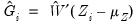 | (60.12) |
where

is a

matrix of factor score coefficients derived from the estimates of the factor model. Often, we will construct estimates using the original data so that

but this is not required; we may for example use coefficients obtained from one set of data to score individuals in a second set of data.
Various methods for estimating the score coefficients

have been proposed. The first class of factor scoring methods computes
exact or
refined estimates of the coefficient weights

. Generally speaking, these methods optimize some property of the estimated scores with respect to the choice of

. For example, Thurstone’s regression approach maximizes the correlation of the scores with the true factors (Gorsuch, 1983). Other methods minimize a function of the estimated errors

with respect to

, subject to constraints on the estimated factor scores. For example, Anderson and Rubin (1956) and McDonald (1981) compute weighted least squares estimators of the factor scores, subject to the condition that the implied correlation structure of the scores

, equals

.
The second set of methods computes
coarse coefficient weights in which the elements of

are restricted to be (-1, 0, 1) values. These simplified weights are determined by recoding elements of the factor loadings matrix or an exact coefficient weight matrix on the basis of their magnitudes. Values of the matrices that are greater than some threshold (in absolute value) are assigned sign-corresponding values of -1 or 1; all other values are recoded at 0 (Grice, 2001).
Score Evaluation
There are an infinite number of factor score estimates that are consistent with an estimated factor model. This lack of identification, termed factor indeterminacy, has received considerable attention in the literature (see for example, Mulaik (1996); Steiger (1979)), and is a primary reason for the multiplicity of estimation methods, and for the development of procedures for evaluating the quality of a given set of scores (Gorsuch, 1983, p. 272).
See Gorsuch (1993) and Grice(2001) for additional discussion of the following measures.
Indeterminacy Indices
There are two distinct types of indeterminacy indices. The first set measures the multiple correlation between each factor and the observed variables,

and its square

. The squared multiple correlations are obtained from the diagonals of the matrix

where

is the observed dispersion matrix and

is the factor structure matrix. Both of these indices range from 0 to 1, with high values being desirable.
The second type of indeterminacy index reports the minimum correlation between alternate estimates of the factor scores,
. The minimum correlation measure ranges from -1 to 1. High positive values are desirable since they indicate that differing sets of factor scores will yield similar results.
Grice (2001) suggests that values for

that do not exceed 0.707 by a significant degree are problematic since values below this threshold imply that we may generate two sets of factor scores that are orthogonal or negatively correlated (Green, 1976).
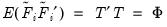
Validity, Univocality, Correlational Accuracy
Following Gorsuch (1983), we may define

as the population factor correlation matrix,

as the factor score correlation matrix, and

as the correlation matrix of the known factors with the score estimates. In general, we would like these matrices to be similar.
The diagonal elements of

are termed
validity coefficients. These coefficients range from -1 to 1, with high positive values being desired. Differences between the validities and the multiple correlations are evidence that the computed factor scores have determinacies lower than those computed using the

-values. Gorsuch (1983) recommends obtaining validity values of at least 0.80, and notes that values larger than 0.90 may be necessary if we wish to use the score estimates as substitutes for the factors.
The off-diagonal elements of

allow us to measure
univocality, or the degree to which the estimated factor scores have correlations with those of other factors. Off-diagonal values of

that differ from those in

are evidence of univocality bias.
Lastly, we obviously would like the estimated factor scores to match the correlations among the factors themselves. We may assess the
correlational accuracy of the scores estimates by comparing the values of the

with the values of

.
From our earlier discussion, we know that the population correlation
.

may be obtained from moments of the estimated scores. Computation of

is more complicated, but follows the steps outlined in Gorsuch (1983).
