Technical Details
The following discussion offers a brief technical summary of GLMs, describing specification, estimation, and hypothesis testing in this framework. Those wishing greater detail should consult the McCullagh and Nelder’s (1989) monograph or the book-length survey by Hardin and Hilbe (2007).
Distribution
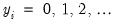
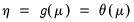
A GLM assumes that

are independent random variables following a linear exponential family distribution with density:
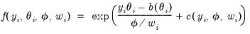 | (32.6) |
where

and

are distribution specific functions.

, which is termed the
canonical parameter, fully parameterizes the distribution in terms of the conditional mean, the
dispersion value

is a possibly known scale nuisance parameter, and

is a known
prior weight that corrects for unequal scaling between observations with otherwise constant

.
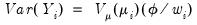
The exponential family assumption implies that the mean and variance of

may be written as
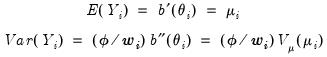 | (32.7) |
where

and

are the first and second derivatives of the

function, respectively, and

is a distribution-specific variance function that depends only on

.
EViews supports the following exponential family distributions:
| | | | |
Normal | | | | |
Gamma | | | | |
Inverse Gaussian | | | | |
Poisson | | | | |
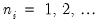
Binomial Proportion (  trials) | | | | |
Negative Binomial (  is known) | | | | |
The corresponding density functions for each of these distributions are given by:
• Normal
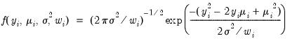 | (32.8) |
for

.
• Gamma
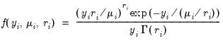 | (32.9) |
for

where

.
• Inverse Gaussian
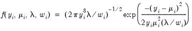 | (32.10) |
for

.
• Poisson
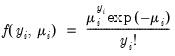 | (32.11) |
for
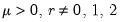
The dispersion is restricted to be

and prior weighting is not permitted.
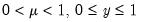
• Binomial Proportion
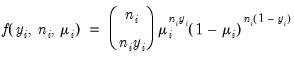 | (32.12) |
for

where
is the number of binomial trials. The dispersion is restricted to be

and the prior weights

.
• Negative Binomial
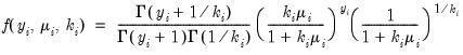 | (32.13) |
for

The dispersion is restricted to be

and prior weighting is not permitted.
In addition, EViews offers support for the following quasi-likelihood families:
| |
Poisson | |
Binomial Proportion | |
Negative Binomial (  ) | |
Power Mean (  ) | |
Exponential Mean | |
Binomial Squared | |
The first three entries in the table correspond to overdispersed or prior weighted versions of the specified distribution. The last three entries are pure quasi-likelihood distributions that do not correspond to exponential family distributions. See
“Quasi-likelihoods” for additional discussion.
Link
The following table lists the names, functions, and associated range restrictions for the supported links:
| | |
Identity | | |
Log | | |
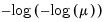
Log-Complement | | |
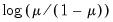
Logit | | |
Probit | | |
Log-Log | | |
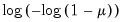
Complementary Log‑Log | | |
Inverse | | |
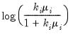
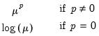
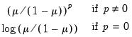
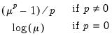
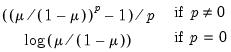
Power (  ) | | |
Power Odds Ratio (  ) | | |
Box-Cox (  ) | | |
Box-Cox Odds Ratio (  ) | | |
EViews does not restrict the link choices associated with a given distributional family. Thus, it is possible for you to choose a link function that returns invalid mean values for the specified distribution at some parameter values, in which case your likelihood evaluation and estimation will fail.
One important role of the inverse link function is to map the real number domain of the linear index into the range of the dependent variable. Consequently the choice of link function is often governed in part by the desire to enforce range restrictions on the fitted mean. For example, the mean of a binomial proportions or negative binomial model must be between 0 and 1, while the Poisson and Gamma distributions require a positive mean value. Accordingly, the use of a Logit, Probit, Log-Log, Complementary Log-Log, Power Odds Ratio, or Box-Cox Odds Ratio is common with a binomial distribution, while the Log, Power, and Box-Cox families are generally viewed as more appropriate for Poisson or Gamma distribution data.
EViews will default to use the
canonical link for a given distribution. The canonical link is the function that equates the canonical parameter

of the exponential family distribution and the linear predictor
. The canonical links for relevant distributions are given by:
| |
Normal | Identity |
Gamma | Inverse |
Inverse Gaussian | Power  |
Poisson | Log |
Binomial Proportion | Logit |
The negative binomial canonical link is not supported in EViews so the log link is used as the default choice in this case. We note that while the canonical link offers computational and conceptual convenience, it is not necessarily the best choice for a given problem.
Quasi-likelihoods
Wedderburn (1974) proposed the method of maximum quasi-likelihood for estimating regression parameters when one has knowledge of a mean-variance relationship for the response, but is unwilling or unable to commit to a valid fully specified distribution function.
Under the assumption that the

are independent with mean

and variance
, the function,
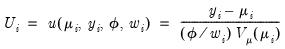 | (32.14) |
has the properties of an individual contribution to a score. Accordingly, the integral,
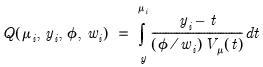 | (32.15) |
if it exists, should behave very much like a log-likelihood contribution. We may use to the individual contributions

to define the
quasi-log-likelihood, and the scaled and unscaled
quasi-deviance functions
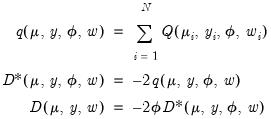 | (32.16) |
We may obtain estimates of the coefficients by treating the quasi-likelihood

as though it were a conventional likelihood and maximizing it respect to

. As with conventional GLM likelihoods, the quasi-ML estimate of

does not depend on the value of the dispersion parameter

. The dispersion parameter is conventionally estimated using the Pearson

statistic, but if the mean-variance assumption corresponds to a valid exponential family distribution, one may also employ the deviance statistic.
For some mean-variance specifications, the quasi-likelihood function corresponds to an ordinary likelihood in the linear exponential family, and the method of maximum quasi-likelihood is equivalent to ordinary maximum likelihood. For other specifications, there is no corresponding likelihood function. In both cases, the distributional properties of the maximum quasi-likelihood estimator will be analogous to those obtained from maximizing a valid likelihood (McCullagh 1983).
We emphasize the fact that quasi-likelihoods offer flexibility in the mean-variance specification, allowing for variance assumptions that extend beyond those implied by exponential family distribution functions. One important example occurs when we modify the variance function for a Poisson, Binomial Proportion, or Negative Binomial distribution to allow a free dispersion parameter.
Furthermore, since the quasi-likelihood framework only requires specification of the mean and variance, it may be used to relax distributional restrictions on the form of the response data. For example, while we are unable to evaluate the Poisson likelihood for non-integer data, there are no such problems for the corresponding quasi-likelihood based on mean-variance equality.
A list of common quasi-likelihood mean-variance assumptions is provided below, along with names for the corresponding exponential family distribution:
| | |
| None | Normal |
| | Poisson |
| | Gamma |
| | --- |
| None | --- |
| | Binomial Proportion |
| | --- |
| | Negative Binomial |
Note that the power-mean

, exponential mean

, and squared binomial proportion

variance assumptions do not correspond to exponential family distributions.
Estimation
Estimation of GLM models may be divided into the estimation of three basic components: the

coefficients, the coefficient covariance matrix

, and the dispersion parameter

.
Coefficient Estimation
The estimation of

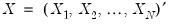
is accomplished using the method of maximum likelihood (ML). Let
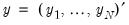
and
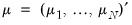
. We may write the log-likelihood function as
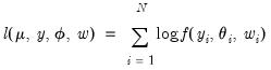 | (32.17) |
Differentiating

with respect to

yields
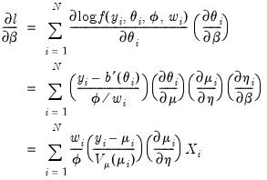 | (32.18) |
where the last equality uses the fact that
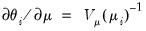
. Since the scalar dispersion parameter

is incidental to the first-order conditions, we may ignore it when estimating

. In practice this is accomplished by evaluating the likelihood function at

.
It will prove useful in our discussion to define the
scaled deviance 
and the
unscaled deviance 
as
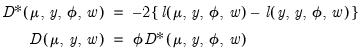 | (32.19) |
respectively. The scaled deviance

compares the likelihood function for the saturated (unrestricted) log-likelihood,

, with the log-likelihood function evaluated at an arbitrary

,

.
The unscaled deviance

is simply the scaled deviance multiplied by the dispersion, or equivalently, the scaled deviance evaluated at

. It is easy to see that minimizing either deviance with respect to

is equivalent to maximizing the log-likelihood with respect to the

.
In general, solving for the first-order conditions for

requires an iterative approach. EViews offers three different algorithms for obtaining solutions: Newton-Raphson, BHHH, and IRLS - Fisher Scoring. All of these methods are variants of Newton’s method but differ in the method for computing the gradient weighting matrix used in coefficient updates (see
“Optimization Algorithms”).
IRLS, which stands for Iterated Reweighted Least Squares, is a commonly used algorithm for estimating GLM models. IRLS is equivalent to Fisher Scoring, a Newton-method variant that employs the Fisher Information (negative of the expected Hessian matrix) as the update weighting matrix in place of the negative of the observed Hessian matrix used in standard Newton-Raphson, or the outer-product of the gradients (OPG) used in BHHH.
In the GLM context, the IRLS-Fisher Scoring coefficient updates have a particularly simple form that may be implemented using weighted least squares, where the weights are known functions of the fitted mean that are updated at each iteration. For this reason, IRLS is particularly attractive in cases where one does not have access to custom software for estimating GLMs. Moreover, in cases where one’s preference is for an observed-Hessian Newton method, the least squares nature of the IRLS updates make the latter well-suited to refining starting values prior to employing one of the other methods.
Coefficient Covariance Estimation
You may choose from a variety of estimators for

, the covariance matrix of

. In describing the various approaches, it will be useful to have expressions at hand for the
expected Hessian (

), the
observed Hessian (

), and the
outer-product of the gradients (

) for GLM models. Let
. Then given estimates of

and the dispersion

(
See “Dispersion Estimation”), we may write
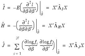 | (32.20) |
where

,

, and

are diagonal matrices with corresponding
i-th diagonal elements
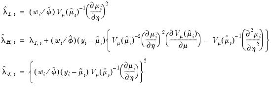 | (32.21) |
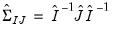
Given correct specification of the likelihood, asymptotically consistent estimators for the

may be obtained by taking the inverse of one of these estimators of the information matrix. In practice, one typically matches the covariance matrix estimator with the method of estimation (
i.e., using the inverse of the expected information estimator

when estimation is performed using IRLS) but mirroring is not required. By default, EViews will pair the estimation and covariance methods, but you are free to mix and match as you see fit.
If the variance function is incorrectly specified, the GLM inverse information covariance estimators are no longer consistent for

. The Huber-White Sandwich estimator (Huber 1967, White 1980) permits non GLM-variances and is robust to misspecification of the variance function. EViews offers two forms for the estimator; you may choose between one that employs the expected information (
) or one that uses the observed Hessian (
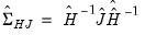
).
Lastly, you may choose to estimate the coefficient covariance with or without a degree-of-freedom correction. In practical terms, this computation is most easily handled by using a non d.f.-corrected version of

in the basic calculation, then multiplying the coefficient covariance matrix by

when you want to apply the correction.
Dispersion Estimation
Recall that the dispersion parameter

may be ignored when estimating

. Once we have obtained

, we may turn attention to obtaining an estimate of

. With respect to the estimation of

, we may divide the distribution families into two classes: distributions with a free dispersion parameter, and distributions where the dispersion is fixed.
For distributions with a free dispersion parameter (Normal, Gamma, Inverse Gaussian), we must estimate

. An estimate of the free dispersion parameter

may be obtained using the generalized Pearson

statistic (Wedderburn 1972, McCullagh 1983),
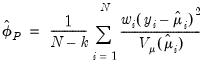 | (32.22) |
where

is the number of estimated coefficients. In linear exponential family settings,

may also be estimated using the unscaled deviance statistic (McCullagh 1983),
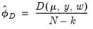 | (32.23) |
For distributions where the dispersion is fixed (Poisson, Binomial, Negative Binomial),

is naturally set to the theoretically proscribed value of 1.0.
In fixed dispersion settings, the theoretical restriction on the dispersion is sometimes violated in the data. This situation is generically termed
overdispersion since

typically exceeds 1.0 (though
underdispersion is a possibility). At a minimum, unaccounted for overdispersion leads to invalid inference, with estimated standard errors of the

typically understating the variability of the coefficient estimates.
The easiest way to correct for overdispersion is by allowing a free dispersion parameter in the variance function, estimating

using one of the methods described above, and using the estimate when computing the covariance matrix as described in
“Coefficient Covariance Estimation”. The resulting covariance matrix yields what are sometimes termed GLM standard errors.
Bear in mind that estimating

given a fixed dispersion distribution violates the assumptions of the likelihood so that standard ML theory does not apply. This approach is, however, consistent with a quasi-likelihood estimation framework (Wedderburn 1974), under which the coefficient estimator and covariance calculations are theoretically justified (see
“Quasi-likelihoods”). We also caution that overdispersion may be evidence of more serious problems with your specification. You should take care to evaluate the appropriateness of your model.
Computational Details
The following provides additional details for the computation of results:
Residuals
There are several different types of residuals that are computed for a GLM specification:
• The ordinary or response residuals are defined as
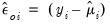 | (32.24) |
The ordinary residuals are simply the deviations from the mean in the original scale of the responses.
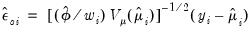
• The weighted or Pearson residuals are given by
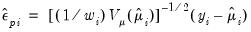 | (32.25) |
The weighted residuals divide the ordinary response variables by the square root of the unscaled variance. For models with fixed dispersion, the resulting residuals should have unit variance. For models with free dispersion, the weighted residuals may be used to form an estimator of

.
• The standardized or scaled Pearson residuals) are computed as
 | (32.26) |
The standardized residuals are constructed to have approximately unit variance.
• The generalized or score residuals are given by
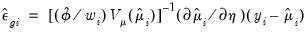 | (32.27) |
The scores of the GLM specification are obtained by multiplying the explanatory variables by the generalized residuals (
Equation (32.18)). Not surprisingly, the generalized residuals may be used in the construction of LM hypothesis tests.
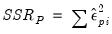
Sum of Squared Residuals
EViews reports two different sums-of-squared residuals: a basic sum of squared residuals,
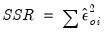
, and the Pearson SSR,
.
Dividing the Pearson SSR by

produces the Pearson

statistic which may be used as an estimator of

, (
“Dispersion Estimation”) and, in some cases, as a measure of goodness-of-fit.
Log-likelihood and Information Criteria
EViews always computes GLM log-likelihoods using the full specification of the density function: scale factors, inessential constants, and all. The likelihood functions are listed in
“Distribution”.
If your dispersion specification calls for a fixed value for

, the fixed value will be used to compute the likelihood. If the distribution and dispersion specification call for

to be estimated,

will be used in the evaluation of the likelihood. If the specified distribution calls for a fixed value for

but you have asked EViews to estimate the dispersion, or if the specified value is not consistent with a valid likelihood, the log-likelihood will not be computed.
The AIC, SIC, and Hannan-Quinn information criteria are computed using the log-likelihood value and the usual definitions (
Appendix E. “Information Criteria”).
It is worth mentioning that computed GLM likelihood value for the normal family will differ slightly from the likelihood reported by the corresponding LS estimator. The GLM likelihood follows convention in using a degree-of-freedom corrected estimator for the dispersion while the LS likelihood uses the uncorrected ML estimator of the residual variance. Accordingly, you should take care not compare likelihood functions estimated using the two methods.
Deviance and Quasi-likelihood
EViews reports the
unscaled deviance

or quasi-deviance. The quasi-deviance and quasi-likelihood will be reported if the evaluation of the likelihood function is invalid. You may divide the reported deviance by

to obtain an estimator of the dispersion, or use the deviance to construct likelihood ratio or
F-tests.
In addition, you may divide the deviance by the dispersion to obtain the scaled deviance. In some cases, the scaled deviance may be used as a measure of goodness-of-fit.
Restricted Deviance and LR Statistic
The restricted deviance and restricted quasi-likelihood reported on the main page are the values for the constant only model.
The entries for “LR statistic” and “Prob(LR statistic)” reported in the output are the corresponding

likelihood ratio tests for the constant only null against the alternative given by the estimated equation. They are the analogues to the “F-statistics” results reported in EViews least squares estimation. As with the latter
F-statistics, the test entries will not be reported if the estimated equation does not contain an intercept.