IV Diagnostics and Tests
EViews offers several IV and GMM specific diagnostics and tests.
Instrument Summary
The Instrument Summary view of an equation is available for non-panel equations estimated by GMM, TSLS or LIML. The summary will display the number of instruments specified, the instrument specification, and a list of the instruments that were used in estimation.
For most equations, the instruments used will be the same as the instruments that were specified in the equation, however if two or more of the instruments are collinear, EViews will automatically drop instruments until the instrument matrix is of full rank. In cases where instruments have been dropped, the summary will list which instruments were dropped.
The Instrument Summary view may be found under .
Instrument Orthogonality Test
The Instrument Orthogonality test, also known as the C-test or Eichenbaum, Hansen and Singleton (EHS) Test, evaluates the othogonality condition of a sub-set of the instruments. This test is available for non-panel equations estimated by TSLS or GMM.
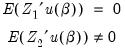
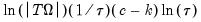
Recall that the central assumption of instrumental variable estimation is that the instruments are orthogonal to a function of the parameters of the model:
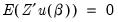 | (23.45) |
The Instrument Orthogonality Test evaluates whether this condition possibly holds for a subset of the instruments but not for the remaining instruments
 | (23.46) |
Where
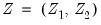
, and

are instruments for which the condition is assumed to hold.
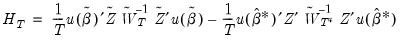
The test statistic,

, is calculated as the difference in
J-statistics between the original equation and a secondary equation estimated using only

as instruments:
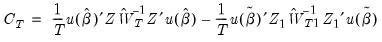 | (23.47) |
where

are the parameter estimates from the original TSLS or GMM estimation, and

is the original weighting matrix,

are the estimates from the test equation, and

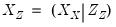
is the matrix for the test equation formed by taking the subset of

corresponding to the instruments in

. The test statistic is Chi-squared distributed with degrees of freedom equal to the number of instruments in

.
To perform the Instrumental Orthogonality Test in EViews, click on . A dialog box will the open up asking you to enter a list of the

instruments for which the orthogonality condition may not hold. Click on and the test results will be displayed.
Regressor Endogeneity Test
The Regressor Endogeneity Test, also known as the Durbin-Wu-Hausman Test, tests for the endogeneity of some, or all, of the equation regressors. This test is available for non-panel equations estimated by TSLS or GMM.
A regressor is endogenous if it is explained by the instruments in the model, whereas exogenous variables are those which are not explained by instruments. In EViews’ TSLS and GMM estimation, exogenous variables may be specified by including a variable as both a regressor and an instrument, whereas endogenous variable are those which are specified in the regressor list only.
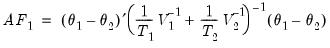
The Endogeneity Test tests whether a subset of the endogenous variables are actually exogenous. This is calculated by running a secondary estimation where the test variables are treated as exogenous rather than endogenous, and then comparing the J-statistic between this secondary estimation and the original estimation:
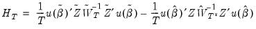 | (23.48) |
where

are the parameter estimates from the original TSLS or GMM estimation obtained using weights

, and

are the estimates from the test equation estimated using

, the instruments augmented by the variables which are being tested, and

is the weighting matrix from the secondary estimation.
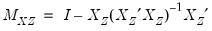
Note that in the case of GMM estimation, the matrix

should be a sub-matrix of

to ensure positivity of the test statistic. Accordingly, in computing the test statistic, EViews first estimates the secondary equation to obtain

, and then forms a new matrix

, which is the subset of

corresponding to the original instruments

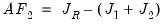
. A third estimation is then performed using the subset matrix for weighting, and the test statistic is calculated as:
 | (23.49) |
The test statistic is distributed as a Chi-squared random variable with degrees of freedom equal to the number of regressors tested for endogeneity.
To perform the Regressor Endogeneity Test in EViews, click on . A dialog box will the open up asking you to enter a list of regressors to test for endogeneity. Once you have entered those regressors, hit and the test results are shown.
Weak Instrument Diagnostics
The Weak Instrument Diagnostics view provides diagnostic information on the instruments used during estimation. This information includes the Cragg-Donald statistic, the associated Stock and Yugo critical values, and Moment Selection Criteria (MSC). The Cragg-Donald statistic and its critical values are available for equations estimated by TSLS, GMM or LIML, but the MSC are available for equations estimated by TSLS or GMM only.
The Cragg-Donald statistic is proposed by Stock and Yugo as a measure of the validity of the instruments in an IV regression. Instruments that are only marginally valid, known as weak instruments, can lead to biased inferences based on the IV estimates, thus testing for the presence of weak instruments is important. For a discussion of the properties of IV estimation when the instruments are weak, see, for example, Moreira 2001, Stock and Yugo 2004 or Stock, Wright and Yugo 2002.
Although the Cragg-Donald statistic is only valid for TSLS and other K-class estimators, EViews also reports for equations estimated by GMM for comparative purposes.
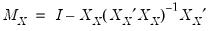
The Cragg-Donald statistic is calculated as:
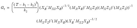 | (23.50) |
where:

= instruments that are not in the regressor list

= exogenous regressors (regressors in both the regressor and instrument lists)

= endogenous regressors (regressors that are not in instrument list)

= number of columns of


= number of columns of

The statistic does not follow a standard distribution, however Stock and Yugo provide a table of critical values for certain combinations of instruments and endogenous variable numbers. EViews will report these critical values if they are available for the specified number of instruments and endogenous variables in the equation.
Moment Selection Criteria (MSC) are a form of Information Criteria that can be used to compare different instrument sets. Comparison of the MSC from equations estimated with different instruments can help determine which instruments perform the best. EViews reports three different MSCs: two proposed by Andrews (1999)—a Schwarz criterion based, and a Hannan-Quinn criterion based, and the third proposed by Hall, Inoue, Jana and Shin (2007)—the Relevant Moment Selection Criterion. They are calculated as follows:
SIC-based =
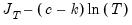
HQIQ-based =
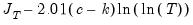
Relevant MSC =
where

= the number of instruments,

= the number of regressors,

= the number of observations,

= the estimation covariance matrix,
and

is equal 1 for TSLS and White GMM estimation, and equal to the bandwidth used in HAC GMM estimation.
To view the Weak Instrument Diagnostics in EViews, click on .
GMM Breakpoint Test
The GMM Breakpoint test is similar to the Chow Breakpoint Test, but it is geared towards equations estimated via GMM rather than least squares.
EViews calculates three different types of GMM breakpoint test statistics: the Andrews-Fair (1988) Wald Statistic, the Andrews-Fair LR-type Statistic, and the Hall and Sen (1999) O-Statistic. The first two statistics test the null hypothesis that there are no structural breaks in the equation parameters. The third statistic tests the null hypothesis that the over-identifying restrictions are stable over the entire sample.
All three statistics are calculated in a similar fashion to the Chow Statistic – the data are partitioned into different subsamples, and the original equation is re-estimated for each of these subsamples. However, unlike the Chow Statistic, which is calculated on the basis that the variance-covariance matrix of the error terms remains constant throughout the entire sample (i.e

. is the same between subsamples), the GMM breakpoint statistic lets the variance-covariance matrix of the error terms vary between the subsamples.
The Andrews-Fair Wald Statistic is calculated, in the single breakpoint case, as:
 | (23.51) |
Where

refers to the coefficient estimates from subsample

,

refers to the number of observations in subsample

, and

is the estimate of the variance-covariance matrix for subsample

.
The Andrews-Fair LR-type statistic is a comparison of the J-statistics from each of the subsample estimations:
 | (23.52) |
Where

is a
J-statistic calculated with the original equation’s residuals, but a GMM weighting matrix equal to the weighted (by number of observations) sum of the estimated weighting matrices from each of the subsample estimations.
The Hall and Sen O-Statistic is calculated as:
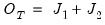 | (23.53) |
The first two statistics have an asymptotic

distribution with

degrees of freedom, where m is the number of subsamples, and k is the number of coefficients in the original equation. The O-statistic also follows an asymptotic

distribution, but with
degrees of freedom.
To apply the GMM Breakpoint test, click on In the dialog box that appears simply enter the dates or observation numbers of the breakpoint you wish to test.