EViews Help: Technical Notes

The default standard errors are obtained by taking the inverse of the estimated information matrix. If you estimate your equation using a Newton-Raphson or Quadratic Hill Climbing method, EViews will use the inverse of the Hessian,

, to form your coefficient covariance estimate. If you employ BHHH, the coefficient covariance will be estimated using the inverse of the outer product of the scores

, where

and

are the gradient (or score) and Hessian of the log likelihood evaluated at the ML estimates.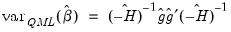

The Huber/White options for robust standard errors computes the quasi-maximum likelihood (or pseudo-ML) standard errors:

The Cluster-robust variants of these errors replace the inner matrix with a cluster-aware version of the moment.

Note that these standard errors are not robust to heteroskedasticity in binary dependent variable models. They are robust to certain misspecifications of the underlying distribution of

, but as with all QML estimation, caution is advised.

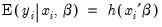
Many of the discrete and limited dependent variable models described in this chapter belong to a class of models known as generalized linear models (GLM). The assumption of GLM is that the distribution of the dependent variable

belongs to the exponential family and that the conditional mean of

is a (smooth) nonlinear transformation of the linear part

Even though the QML covariance is robust to general misspecification of the conditional distribution of

, it does not possess any efficiency properties. An alternative consistent estimate of the covariance is obtained if we impose the GLM condition that the (true) variance of

is proportional to the variance of the distribution used to specify the log likelihood:

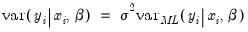
In other words, the ratio of the (conditional) variance to the mean is some constant

that is independent of

. The most empirically relevant case is

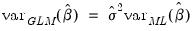
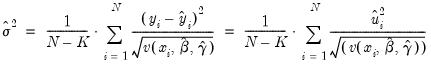
, which is known as overdispersion. If this proportional variance condition holds, a consistent estimate of the GLM covariance is given by:

If you do not choose to d.f. correct, the leading term in Equation (31.66) is

. When you select GLM standard errors, the estimated proportionality term

is reported as the variance factor estimate in EViews.

(Note that the EViews legacy estimator always estimates a d.f. corrected variance factor, while the other estimators permit you to choose whether to override the default of no correction. Since the default behavior has changed, you will need to explicitly request d.f. correction to match the legacy covariance results.)

For detailed discussion on GLMs and the phenomenon of overdispersion, see McCullaugh and Nelder (1989).

Let the data be grouped into

groups, and let

be the number of observations in group

. Define the number of

observations and the average of predicted values in group

as:

The distribution of the HL statistic is not known; however, Hosmer and Lemeshow (1989, p.141) report evidence from extensive simulation indicating that when the model is correctly specified, the distribution of the statistic is well approximated by a

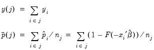
distribution with

degrees of freedom. Note that these findings are based on a simulation where

is close to

Let the data be grouped into

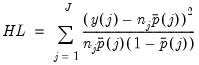
groups. Since

is binary, there are

cells into which any observation can fall. Andrews (1988a, 1988b) compares the

vector of the actual number of observations in each cell to those predicted from the model, forms a quadratic form, and shows that the quadratic form has an asymptotic

distribution if the model is specified correctly.

Andrews suggests three tests depending on the choice of the weighting matrix in the quadratic form. EViews uses the test that can be computed by an auxiliary regression as described in Andrews (1988a, 3.18) or Andrews (1988b, 17).

Briefly, let