Truncated Regression Models
A close relative of the censored regression model is the truncated regression model. Suppose that an observation is not observed whenever the dependent variable falls below one threshold, or exceeds a second threshold. This sampling rule occurs, for example, in earnings function studies for low-income families that exclude observations with incomes above a threshold, and in studies of durables demand among individuals who purchase durables.
The general two-limit truncated regression model may be written as:
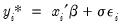 | (31.32) |
where

is only observed if:
 | (31.33) |
If there is no lower truncation, then we can set

. If there is no upper truncation, then we set

.
The log likelihood function associated with these data is given by:
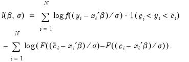 | (31.34) |
The likelihood function is maximized with respect to

and

, using standard iterative methods.
Estimating a Truncated Model in EViews
Estimation of a truncated regression model follows the same steps as estimating a censored regression:
• Select from the main menu, and in the Equation Specification dialog, select the CENSORED estimation method. The censored and truncated regression dialog will appear.
• Enter the name of the truncated dependent variable and the list of the regressors or provide explicit expression for the equation in the Equation Specification field, and select one of the three distributions for the error term.
• Indicate that you wish to estimate the truncated model by checking the Truncated sample option.
• Specify the truncation points of the dependent variable by entering the appropriate expressions in the two edit fields. If you leave an edit field blank, EViews will assume that there is no truncation along that dimension.
You should keep a few points in mind. First, truncated estimation is only available for models where the truncation points are known, since the likelihood function is not otherwise defined. If you attempt to specify your truncation points by index, EViews will issue an error message indicating that this selection is not available.
Second, EViews will issue an error message if any values of the dependent variable are outside the truncation points. Furthermore, EViews will automatically exclude any observations that are exactly equal to a truncation point. Thus, if you specify zero as the lower truncation limit, EViews will issue an error message if any observations are less than zero, and will exclude any observations where the dependent variable exactly equals zero.
The cumulative distribution function and density of the assumed distribution will be used to form the likelihood function, as described above.
Procedures for Truncated Equations
EViews provides the same procedures for truncated equations as for censored equations. The residual and forecast calculations differ to reflect the truncated dependent variable and the different likelihood function.
Make Residual Series
Select , and select from among the three types of residuals. The three types of residuals for censored models are defined as:
Ordinary | |
Standardized | |
Generalized | |
where

,

, are the density and distribution functions. Details on the computation of
are provided below.
The generalized residuals may be used as the basis of a number of LM tests, including LM tests of normality (see Chesher and Irish (1984, 1987), and Gourieroux, Monfort and Trognon (1987); Greene (2008) provides a brief discussion and additional references).
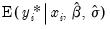
Forecasting
EViews provides you with the option of forecasting the expected observed dependent variable,
, or the expected latent variable,
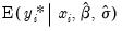
.
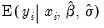
To forecast the expected latent variable, select from the equation toolbar to open the forecast dialog, click on
Index - Expected latent variable, and enter a name for the series to hold the output. The forecasts of the expected latent variable
are computed using:
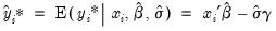 | (31.35) |
where

is the Euler-Mascheroni constant (
).
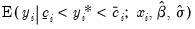
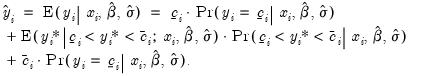
To forecast the expected observed dependent variable for the truncated model, you should select Expected dependent variable, and enter a series name. These forecasts are computed using:
 | (31.36) |
so that the expectations for the latent variable are taken with respect to the conditional (on being observed) distribution of the

. Note that these forecasts always satisfy the inequality

.
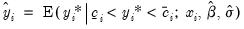
It is instructive to compare this latter expected value with the expected value derived for the censored model in
Equation (31.30) above (repeated here for convenience):
 | (31.37) |
The expected value of the dependent variable for the truncated model is the first part of the middle term of the censored expected value. The differences between the two expected values (the probability weight and the first and third terms) reflect the different treatment of latent observations that do not lie between

and

. In the censored case, those observations are included in the sample and are accounted for in the expected value. In the truncated case, data outside the interval are not observed and are not used in the expected value computation.
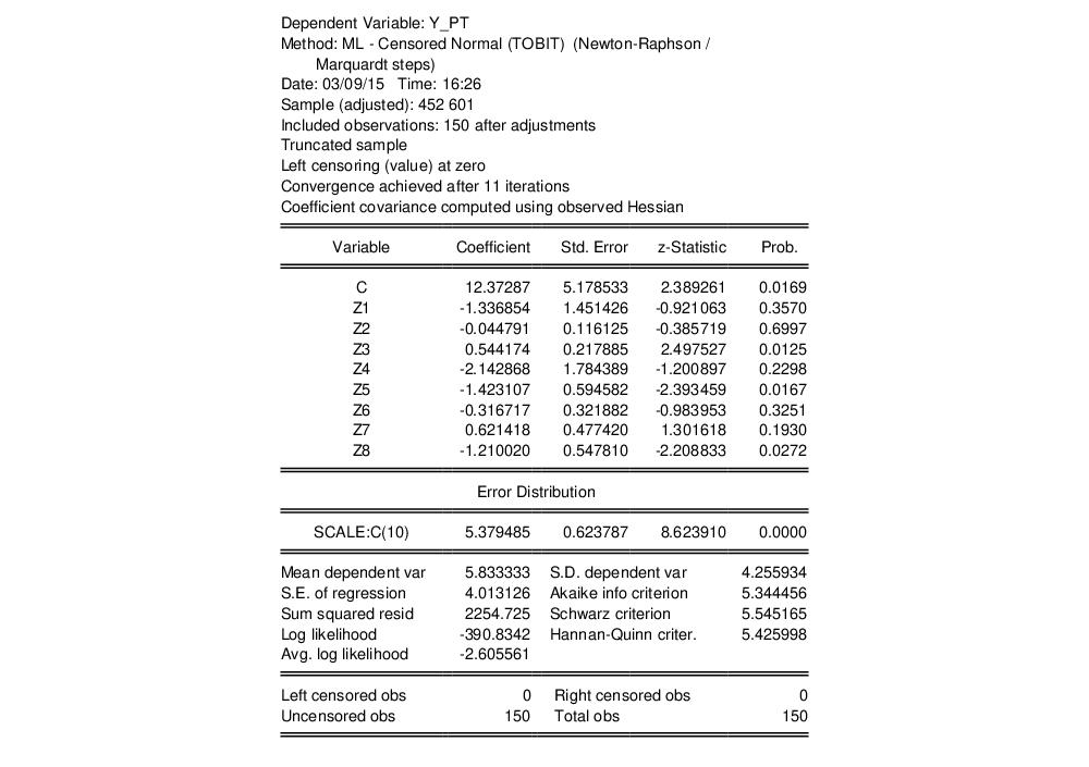
An Illustration
As an example, we reestimate the Fair tobit model from above, truncating the data so that observations at or below zero are removed from the sample. The output from truncated estimation of the Fair model is presented below:
Note that the header information indicates that the model is a truncated specification with a sample that is adjusted accordingly, and that the frequency information at the bottom of the screen shows that there are no left and right censored observations.