The VAR contains  variables
  , observed at low frequency and
  variables
  observed at the high frequency. Let
variables , observed at low frequency and variables observed at the high frequency. Let variables , observed at low frequency and variables observed at the high frequency. Let  represent the i-th low frequency variable observed during low-frequency period
 represent the i-th high frequency variable observed in the t-th high-frequency period during low-frequency period
 and
and  variables into the matrices
  and
and  , respectively, and for brevity ignoring the intercepts and exogenous variables, we may write the VAR as:
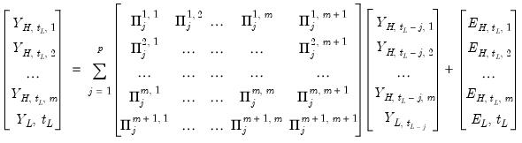 | (49.1) |
 is
is  ,
,  is
is  , and
, and  is
is  , for all
  ,
, 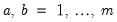 , and
, and  is
is  .
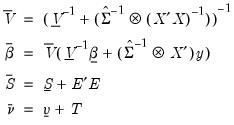
. , the stacked matrix of coefficients.
 and the residual covariance matrix,
  (
“Technical Background”).
(
“Technical Background”).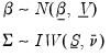 | (49.2) |
 and
and  of:
of: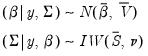 | (49.3) |
(49.4) |
 | (49.5) |
 is constructed like the Litterman prior in standard Bayesian VARs.
  is assumed to be all zero, other than the own first lag terms. However the Ghysels prior differs slightly by allowing a different hyper-parameter for the own lag term depending on whether a variable is high or low frequency. Another crucial difference is that the variables are assumed to follow an AR(1) process in the high-frequency, so that when estimating in low-frequency space, the parameter is exponential.
 is similar to a Litterman prior, but with subtle differences to allow for the cross-frequency variances.
 Element | Mean | Variance | Dimension |
 |  |  |  , ,  |
 |  |  |  |
 | 0 | 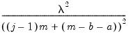 |  , ,  , ,  |
 | 0 | 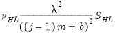 |  , ,  |
 | 0 | 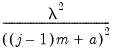 |  , ,  , ,  |
 | 0 |  |  , ,  |
 | 0 |  |  , ,  |
 ,
,  ,
,  and
and  are hyper-parameters, and
  is a
is a  matrix with the (i,j)-th element equal to
  ,
,  ,
,  where the
  are taken from a univariate AR(1) estimation.
 .
. is formed by taking a scaled identity matrix or by scaling an initial estimate of the variance taken from a classical least squares U-MIDAS estimation:
 | (49.6) |
 or
or  .
.