Panel Estimation Examples
Least Squares Examples
To illustrate the estimation of panel equations in EViews, we first consider an example involving unbalanced panel data from Harrison and Rubinfeld (1978) for the study of hedonic pricing (“Harrison_panel.WF1”). The data are well known and used as an example dataset in many sources (e.g., Baltagi (2005), p. 171).
The data consist of 506 census tract observations on 92 towns in the Boston area with group sizes ranging from 1 to 30. The dependent variable of interest is the logarithm of the median value of owner occupied houses (MV), and the regressors include various measures of housing desirability.
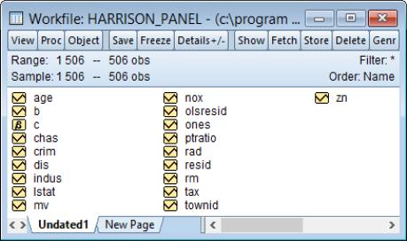
We begin our example by structuring our workfile as an undated panel. Click on the “Range:” description in the workfile window, select , and enter “TOWNID” as the . EViews will prompt you twice to create a CELLID series to uniquely identify observations. Click on to both questions to accept your settings.
EViews restructures your workfile so that it is an unbalanced panel workfile. The top portion of the workfile window will change to show the undated structure which has 92 cross-sections and a maximum of 30 observations in a cross-section.
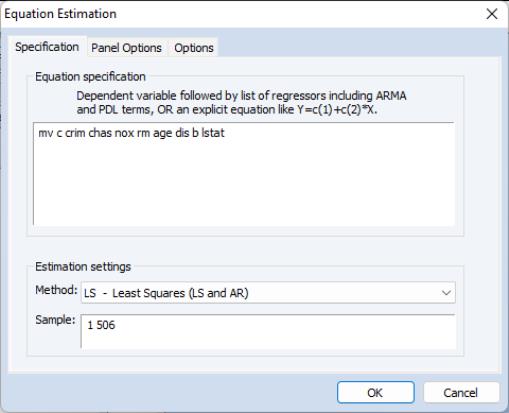
Next, we open the equation specification dialog by selecting from the main EViews menu.
First, following Baltagi and Chang (1994) (also described in Baltagi, 2005), we estimate a fixed effects specification of a hedonic housing equation. The dependent variable in our specification is the median value MV, and the regressors are the crime rate (CRIM), a dummy variable for the property along Charles River (CHAS), air pollution (NOX), average number of rooms (RM), proportion of older units (AGE), distance from employment centers (DIS), proportion of African-Americans in the population (B), and the proportion of lower status individuals (LSTAT). Note that you may include a constant term C in the specification. Since we are estimating a fixed effects specification, EViews will add one if it is not present so that the fixed effects estimates are relative to the constant term and add up to zero.
Click on the tab and select for the effects. To match the Baltagi and Chang results, we will leave the remaining settings at their defaults. Click on to accept the specification.
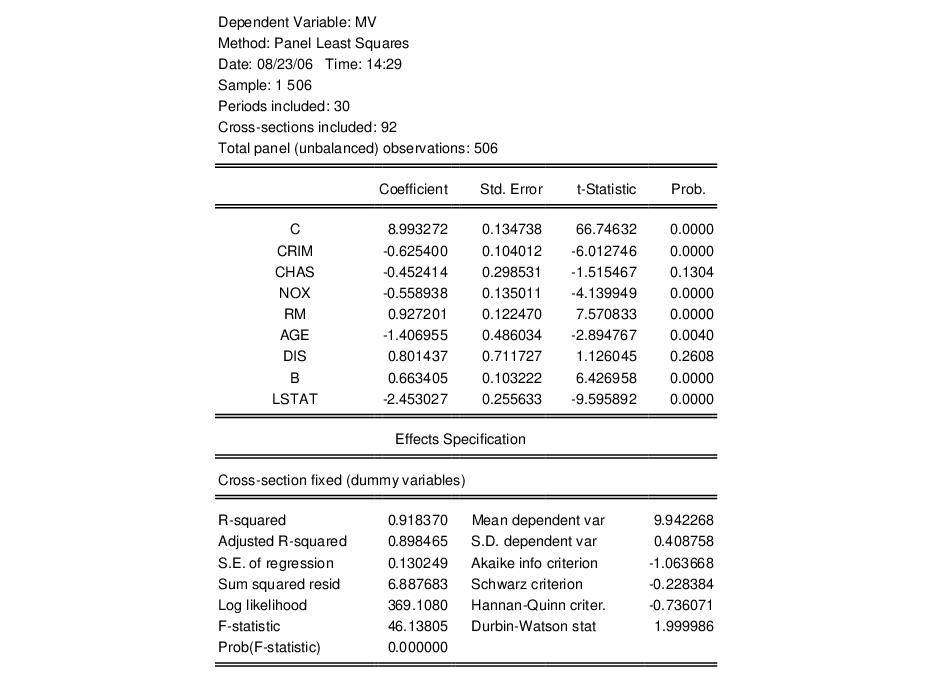
The results for the fixed effects estimation are depicted here. Note that as in pooled estimation, the reported R-squared and F-statistics are based on the difference between the residuals sums of squares from the estimated model, and the sums of squares from a single constant-only specification, not from a fixed-effect-only specification. Similarly, the reported information criteria report likelihoods adjusted for the number of estimated coefficients, including fixed effects. Lastly, the reported Durbin-Watson stat is formed simply by computing the first-order residual correlation on the stacked set of residuals.
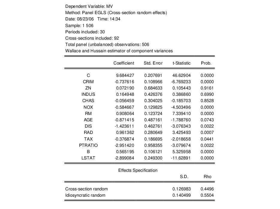
We may click on the button to modify the specification to match the Wallace-Hussain random effects specification considered by Baltagi and Chang. We modify the specification to include the additional regressors (ZN, INDUS, RAD, TAX, PTRATIO) used in estimation, change the cross-section effects to be estimated as a random effect, and use the page to set the random effects computation method to Wallace-Hussain.
The top portion of the resulting output is given by:
Note that the estimates of the component standard deviations must be squared to match the component variances reported by Baltagi and Chang (0.016 and 0.020, respectively).
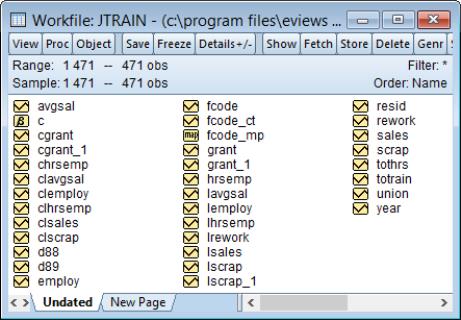
Next, we consider an example of estimation with standard errors that are robust to serial correlation. For this example, we employ data on job training grants (“Jtrain.WF1”) used in examples from Wooldridge (2002, p. 276 and 282).
As before, the first step is to structure the workfile as a panel workfile. Click on to bring up the dialog, and enter “YEAR” as the date identifier and “FCODE” as the cross-section ID.
EViews will structure the workfile so that it is a panel workfile with 157 cross-sections, and three annual observations. Note that even though there are 471 observations in the workfile, a large number of them contain missing values for variables of interest.
To estimate the fixed effect specification with robust standard errors (Wooldridge example 10.5, p. 276), click on specification from the main EViews menu. Enter the list specification:
lscrap c d88 d89 grant grant_1
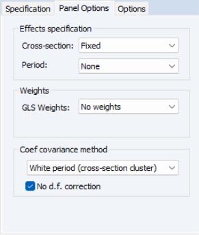
in the edit box on the main page and select in the Cross-section effects specification dropdown menu on the page.
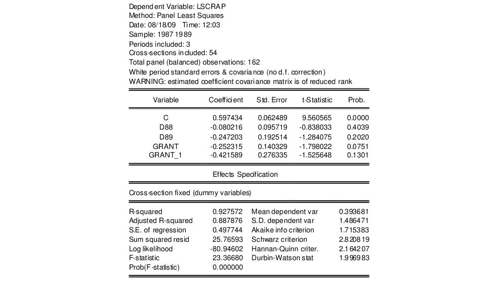
Lastly, since we wish to compute standard errors that are robust to serial correlation (Arellano (1987), White (1980)), we choose as the . To match the reported Wooldridge example, we must select in the covariance calculation. Click on to accept the options. EViews displays the results from estimation:
Note that EViews automatically adjusts for the missing values in the data. There are only 162 observations on 54 cross-sections used in estimation. The top portion of the output indicates that the results use robust White period standard errors with no d.f. correction. Notice that EViews warns you that the estimated coefficient covariances is not of full rank which occurs in this case since the number of periods is less than the number of cross-sections.
Alternately, we may estimate a first difference estimator for these data with robust standard errors (Wooldridge example 10.6, p. 282). Open a new equation dialog by clicking on , or modify the existing equation by clicking on the button on the equation toolbar. Enter the specification:
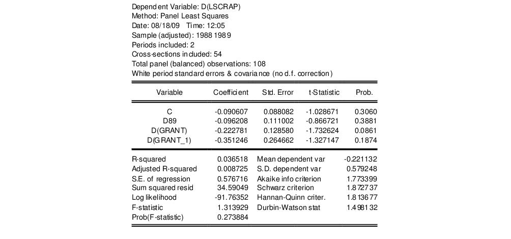
d(lscrap) c d89 d(grant) d(grant_1)
in the edit box on the main page, select in the Cross-section effects specification dropdown menu, and for the coefficient covariance method on the page. The results are given by:
While current versions of EViews do not provide a full set of specification tests for panel equations, it is a straightforward task to construct some tests using residuals obtained from the panel estimation.
To continue with the Wooldridge example, we may test for AR(1) serial correlation in the first-differenced equation by regressing the residuals from this specification on the lagged residuals using data for the year 1989. First, we save the residual series in the workfile. Click on on the estimated equation toolbar, and save the residuals to the series RESID01.
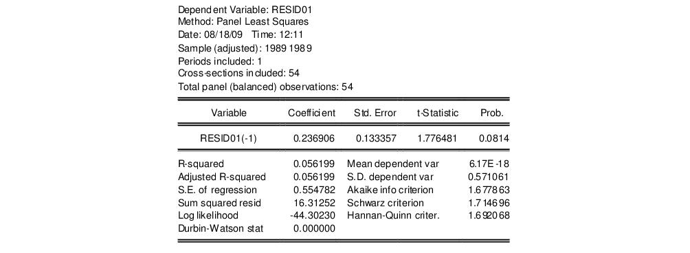
Next, regress RESID01 on RESID01(-1), yielding:
Under the null hypothesis that the original idiosyncratic errors are uncorrelated, the residuals from this equation should have an autocorrelation coefficient of -0.5. Here, we obtain an estimate of

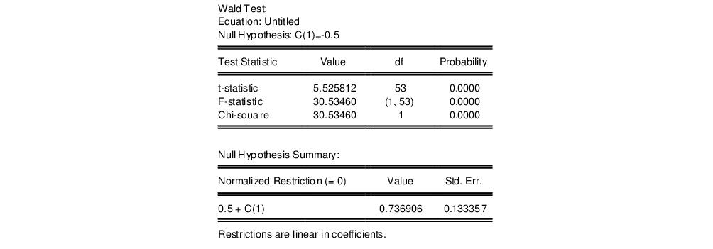
which appears to be far from the null value. A formal Wald hypothesis test rejects the null that the original idiosyncratic errors are serially uncorrelated. Perform a Wald test on the test equation by clicking on and entering the restriction “C(1)=-0.5” in the edit box:
The formal test confirms our casual observation, strongly rejecting the null hypothesis.
Instrumental Variables Example
To illustrate the estimation of instrumental variables panel estimators, we consider an example taken from Papke (1994) for enterprise zone data for 22 communities in Indiana that is outlined in Wooldridge (2002, p. 306).
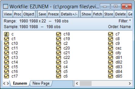
The panel workfile for this example is structured using YEAR as the period identifier, and CITY as the cross-section identifier. The result is a balanced annual panel for dates from 1980 to 1988 for 22 cross-sections.
To estimate the example specification, create a new equation by entering the keyword tsls in the command line, or by clicking on in the main menu. Selecting in the dropdown menu to display the instrumental variables estimator dialog, if necessary, and enter:
d(luclms) c d(luclms(-1)) d(ez)
to regress the difference of log unemployment claims (LUCLMS) on the lag difference, and the difference of enterprise zone designation (EZ). Since the model is estimated with time intercepts, you should click on the page, and select for the effects.
Next, click on the Instruments tab, and add the names:
c d(luclms(-2)) d(ez)
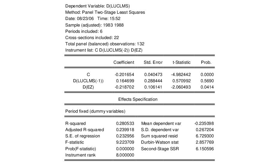
to the edit box. Note that adding the constant C to the regressor and instrument boxes is not required since the fixed effects estimator will add it for you. Click on to accept the dialog settings. EViews displays the output for the IV regression:
Note that the instrument rank in this equation is 8 since the period dummies also serve as instruments, so you have the 3 instruments specified explicitly, plus 5 for the non-collinear period dummy variables.
GMM Example
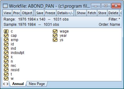
To illustrate the estimation of dynamic panel data models using GMM, we employ the unbalanced 1031 observation panel of firm level data (“Abond_pan.WF1”) from Layard and Nickell (1986), previously examined by Arellano and Bond (1991). The analysis fits the log of employment (N) to the log of the real wage (W), log of the capital stock (K), and the log of industry output (YS).
The workfile is structured as a dated annual panel using ID as the cross-section identifier series and YEAR as the date classification series.
Since the model is assumed to be dynamic, we employ EViews tools for estimating dynamic panel data models. To bring up the GMM dialog, enter the keyword gmm in the command line, or select from the main menu, and choose in the dropdown menu to display the IV estimator dialog.
Click on the button labeled to bring up the DPD wizard. The DPD wizard is a tool that will aid you in filling out the general GMM dialog. The first page is an introductory screen describing the basic purpose of the wizard. Click to continue.
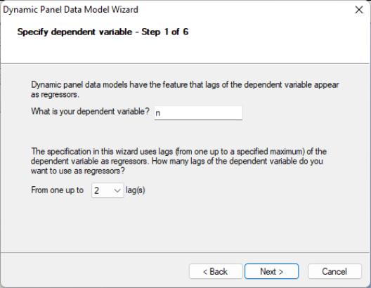
The second page of the wizard prompts you for the dependent variable and the number of its lags to include as explanatory variables. In this example, we wish to estimate an equation with N as the dependent variable and N(-1) and N(-2) as explanatory variables so we enter “N” and select “2” lags in the dropdown menu. Click on to continue to the next page, where you will specify the remaining explanatory variables.
In the next page, you will complete the specification of your explanatory variables. First, enter the list:
w w(-1) k ys ys(-1)
in the regressor edit box to include these variables. Since the desired specification will include time dummies, make certain that the checkbox for is selected, then click on to proceed.
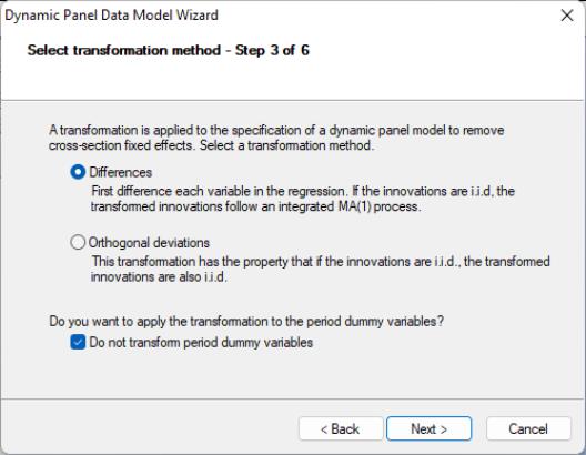
The next page of the wizard is used to specify a transformation to remove the cross-section fixed effect. You may choose to use first or . In addition, if your specification includes period dummy variables, there is a checkbox asking whether you wish to transform the period dummies, or to enter them in levels. Here we specify the first difference transformation, and choose to include untransformed period dummies in the transformed equation. Click on to continue.
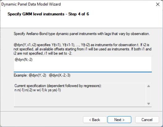
The next page is where you will specify your dynamic period-specific (predetermined) instruments. The instruments should be entered with the “@DYN” tag to indicate that they are to be expanded into sets of predetermined instruments, with optional arguments to indicate the lags to be included. If no arguments are provided, the default is to include all valid lags (from -2 to “-infinity”). Here, we instruct EViews that we wish to use the default lags for N as predetermined instruments.
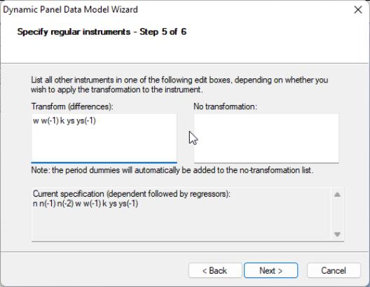
You should now specify the remaining instruments. There are two lists that should be provided. The first list, which is entered in the edit field labeled , should contain a list of the strictly exogenous instruments that you wish to transform prior to use in estimating the transformed equation. The second list, which should be entered in the edit box should contain a list of instruments that should be used directly without transformation. Enter the remaining instruments:
w w(-1) k ys ys(-1)
in the first edit box and click on to proceed to the final page.
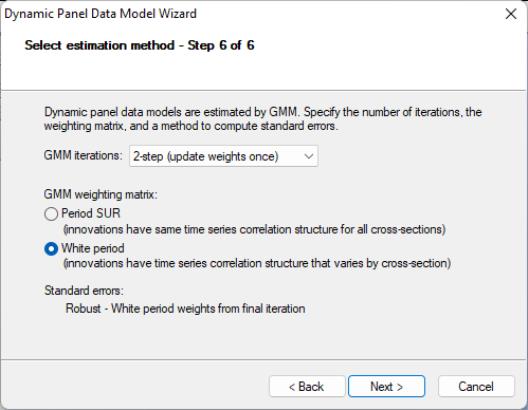
The final page allows you to specify your GMM weighting and coefficient covariance calculation choices. In the first dropdown menu, you will choose a GMM Iteration option. You may select to compute the Arellano-Bond 1-step estimator, to compute the Arellano-Bond 2-step estimator, , to iterate the weight calculations. In the first case, EViews will provide you with choices for computing the standard errors, but here only White period robust standard errors are allowed. Clicking on takes you to the final page. Click on to return to the dialog.
EViews has filled out the dialog with our choices from the DPD wizard. You should take a moment to examine the settings that have been filled out for you since, in the future, you may wish to enter the specification directly into the dialog without using the wizard. You may also, of course, modify the settings in the dialog prior to continuing. For example, click on the tab and check the setting in the covariance calculation to match the original Arellano-Bond results (Table 4(b), p. 290). Click on to estimate the specification.
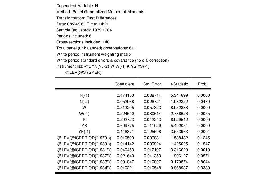
The top portion of the output describes the estimation settings, coefficient estimates, and summary statistics. Note that both the weighting matrix and covariance calculation method used are described in the top portion of the output.
The standard errors that we report here are the standard Arellano-Bond 2-step estimator standard errors. Note that there is evidence in the literature that the standard errors for the two-step estimator may not be reliable.
The bottom portion of the output displays additional information about the specification and summary statistics:
Note in particular the results labeled “J-statistic” and “Instrument rank”. Since the reported J-statistic is simply the Sargan statistic (value of the GMM objective function at estimated parameters), and the instrument rank of 38 is greater than the number of estimated coefficients (13), we may use it to construct the Sargan test of over-identifying restrictions. It is worth noting here that the J-statistic reported by a panel equation differs from that reported by an ordinary equation by a factor equal to the number of observations. Under the null hypothesis that the over-identifying restrictions are valid, the Sargan statistic is distributed as a

, where

is the number of estimated coefficients and

is the instrument rank. The
p-value of 0.22 in this example may be computed using “scalar pval = @chisq(30.11247, 25)”.
Pooled Mean Group Example
As an example of the pooled mean group estimator, we follow the application given in PSS estimating consumption functions for OECD countries in the years 1962–1993. The data are in the file “OECD.wf1”. The series CONS contains per capita real private consumption for each country. INF is a measure of inflation, and INC is per capita real disposable income. PSS estimate an ARDL(1,1,1) model with the natural log of CONS as the dependent variable and the logs of INF and INC as the two dynamic regressors, with a constant as a static regressor.
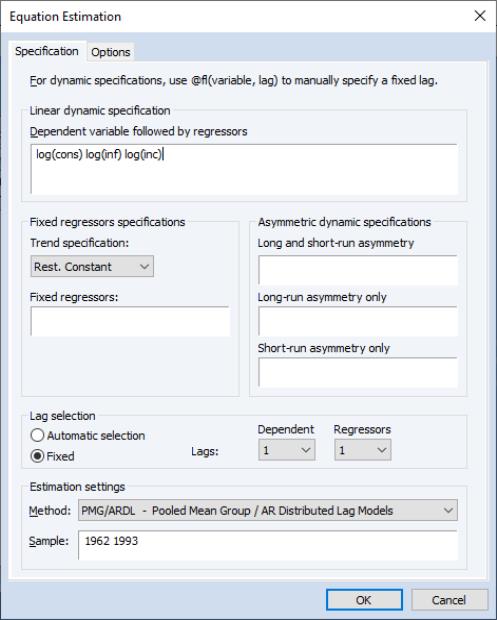
We can estimate this in EViews by clicking on and then selecting PMG/ARDL in the method dropdown. We enter
log(cons) log(inf) log(inc)
in the Dynamic Specification box, select the Fixed radio button to turn off model selection, and change the number of dependent lags and regressor lags to 1. To match PSS, we change the estimation sample to “1962 1993”. Leaving all other options at their default values, we click OK to estimate the model.
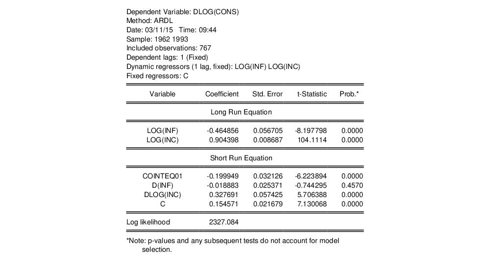
The results are as shown:
The first part of the output gives a summary of the settings used in estimation. The table that follows is split into two blocks. The first block displays estimates of the long-run or pooled coefficients. The second block includes estimates for the mean-group coefficients.
The coefficient on the log of inflation is an estimate of the long-run inflation elasticity, and is negative (and strongly significant), as economic theory, and PSS, expect. We would expect the long run income elasticity (the coefficient on the log of income) to be equal to one, but the estimated value is slightly less at 0.904.
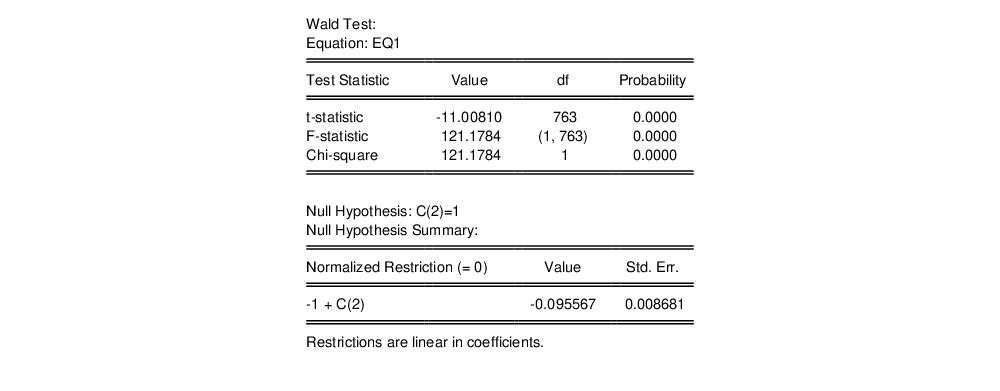
We can perform a Wald test of unit elasticity by clicking on , and entering the restriction of C(2)=1. This test rejects the null hypothesis of unit elasticity.
Click on to display the error correction results for each cross-section:
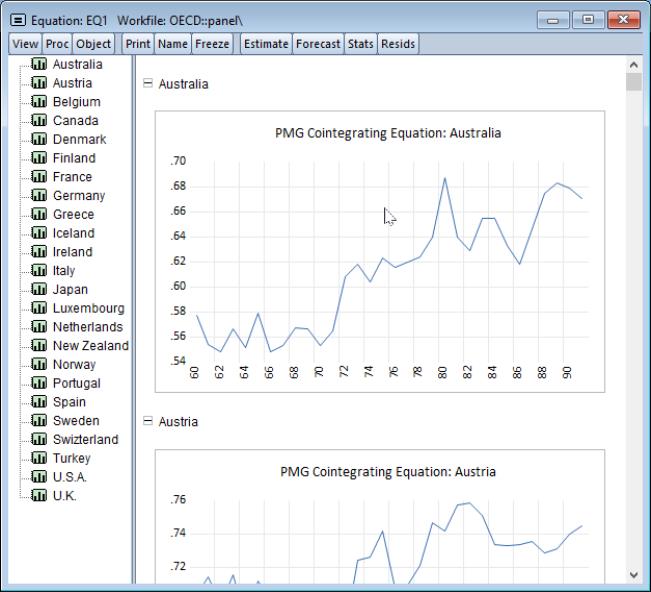
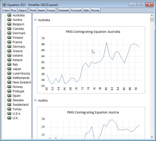
and to display the cointegrating series,



 which appears to be far from the null value. A formal Wald hypothesis test rejects the null that the original idiosyncratic errors are serially uncorrelated. Perform a Wald test on the test equation by clicking on View/Coefficient Diagnostics/Wald-Coefficient Restrictions... and entering the restriction “C(1)=-0.5” in the edit box:

 , where
  is the number of estimated coefficients and
  is the instrument rank. The p-value of 0.22 in this example may be computed using “scalar pval = @chisq(30.11247, 25)”.