Panel Covariances
Panel structured data employ more than one dimension to identify a given observation. In the most common case where the panel combines time series and cross-sectional data, we have data for cross-section units

and periods

. In this setting, we focus on a single random variable

, with individual observations denoted

.
It is sometimes convenient to view the

for different cross-sections (or time periods) as being distinct random variables. This unstacking of a single random variable into multiple random variables permits us to define measures of association between cross-sections or periods for a given panel series.
For example, we may define the
contemporaneous or
between cross-section covariances for

:
 | (58.1) |
where

is the random variable associated with the

for the
i-th cross-section,

. The contemporaneous covariances are a measure of association (dependence) between the data for different cross-sections at a given point in time.
Similarly, we may define the
period or
within cross-section covariances for

:
 | (58.2) |
where

,

. The within cross-section covariances measure the association between the data in different periods for a given cross-section.
Panel covariances and correlations are widely used in panel data analysis. For example:
• Contemporaneous correlations between macroeconomic variables are often used to examine the nature of relationships between different countries (see for example, Obstfeld and Rogoff, 2001, p. 368).
• The contemporaneous covariances of residuals from panel regression are used in computing cross-sectional Zellner SUR-type estimators (Johnston and Dinardo, 1997, p. 318) and in tests of cross-section dependence (Pesaran, 2004). Similarly, panel covariances are used as a first step in obtaining common factors for unit root and other tests (Bai and Ng, 2004).
• Analogously, period covariances of residuals may be used to compute feasible GLS estimators that correct for within cross-section (cluster) correlation.
Once we unstack the data, the computation of estimates of panel measures of association for a single series follows the standard methods (cross-reference to groups). For example, the standard Pearson estimators for the contemporaneous cross-section covariance use variation across time to obtain estimates:
 | (58.3) |
where

and

.
The corresponding Pearson estimators of the period covariances use variation in the cross-section dimension to provide estimates:
 | (58.4) |
where

and

.
Other measures of association may be defined similarly. For discussion of the various methods that EViews supports, see
“Covariance Analysis”.
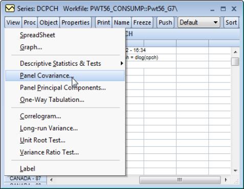
Telling EViews to compute measures of association for a series in a panel structured workfile is straightforward. Simply open the series, and select to display the dialog. Note that the workfile must be structured as a panel for the panel covariance menu entry to be available.
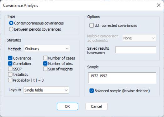
EViews will open the dialog which provides options for controlling the computation, display, and saving of results.
For the most part, the dialog is unchanged from the covariance dialog for a group of series and the discussion of settings there is directly relevant (see
“Covariance Analysis”).
The one notable difference in the current dialog are the radio buttons that allow you to choose whether to compute or .
By changing the settings in the portion dialog, you may instruct EViews to compute a variety of other measures of association (uncentered Pearson, Spearman rank correlations and Kendall’s tau), as well as test statistics for whether the measure of association is zero.
In addition, you may specify a sample to be used in computation and select whether you wish EViews to employ listwise deletion to balance the sample in the event that there are missing values in the series. If you will be working with series with missing observations you should bear in mind that:
• EViews will compute covariances for all of the cross-sections (for contemporaneous covariances) or periods (for between-period covariances) in the specified sample, even if there are no valid observations for a relevant cross-section or period. If you wish to exclude periods or cross-sections from the analysis, you should do so by setting the sample.
• For cross-section covariances, checking the setting instructs EViews to balance the data by removing data for periods where there are missing values for any cross-section.
• For period covariances, the setting will remove data for entire cross-sections where there are missing observations for any period.
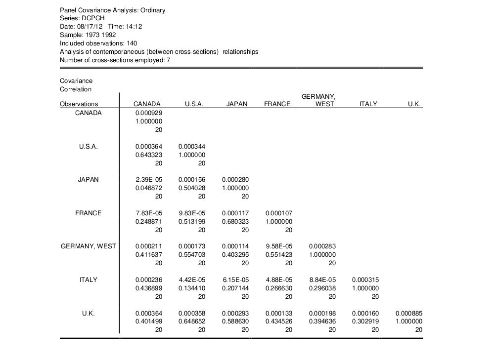
To illustrate, we follow Obstfeld and Rogoff (2001) in computing the cross-country correlations for per capita consumption growth (DCPCH) for the Group of Seven countries over the period from 1973 to 1992. The data, which are from the Penn World Table 5.6, are provided for you in the workfile “PWT56_CONSUMP.wf1” in the Example Files folder in your EViews installation directory.
Open the workfile and the series DCPCH, select and fill in the dialog as depicted above. Click on to compute the requested statistics and display the results.
These results show the correlations in the values of DCPCH between cross-sections.
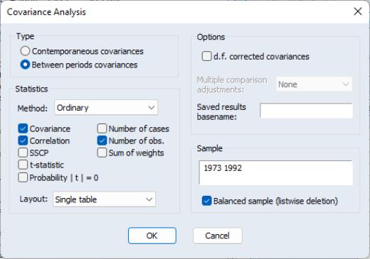
Likewise, we may instruct EViews to compute the between period covariances, we obtain correlations between periods. Fill in the dialog as in the previous example, changing the to , and change the sample to “1973 1992” since data for DCPCH in 1972 are not available (due to the lag in the difference).
If you were to use the original sample of “1972 1992” the resulting between period correlation matrix would contain only NAs (since the balanced sample option would remove all observations). Click on to accept the settings and compute the between covariances and correlations.
 and periods
  . In this setting, we focus on a single random variable
  , with individual observations denoted
  .
. and periods
  . In this setting, we focus on a single random variable
  , with individual observations denoted
  .
. for different cross-sections (or time periods) as being distinct random variables. This unstacking of a single random variable into multiple random variables permits us to define measures of association between cross-sections or periods for a given panel series.
 :
:
 is the random variable associated with the
  for the
  . The contemporaneous covariances are a measure of association (dependence) between the data for different cross-sections at a given point in time.
  :
:
 ,
,  . The within cross-section covariances measure the association between the data in different periods for a given cross-section.
 and
and  .
.
 and
and  .
.


