(33.1)
| (33.1) |
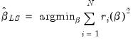
 is given by
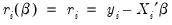 | (33.2) |
 enter the objective function on the right-hand side of
Equation (33.1) after squaring, the effects of outliers are magnified accordingly.
enter the objective function on the right-hand side of
Equation (33.1) after squaring, the effects of outliers are magnified accordingly.  of the residuals:
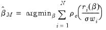 | (33.3) |
 is a measure of the scale of the residuals,
  is an arbitrary positive tuning constant associated with the function, and where
  are individual weights that are generally set to 1, but may be set to:
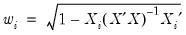 | (33.4) |
 (Andrews, Bisquare, Cauchy, Fair, Huber-Bisquare, Logistic, Median, Talworth, Welsch) are outlined below along with the default values of the tuning constants:
Name |  | Default  |
Andrews | 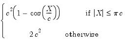 | 1.339 |
Bisquare | 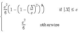 | 4.685 |
Cauchy | 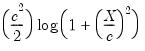 | 2.385 |
Fairl | 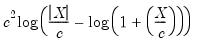 | 1.4 |
Huber | 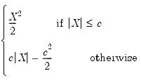 | 1.345 |
Logistic |  | 1.205 |
Median |  | 0.01 |
Talworth |  | 2.796 |
Welsch | 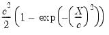 | 2.985 |
 is known, then the
  -vector of coefficient estimates
  may be found using standard iterative techniques for solving the
  nonlinear first-order equations:
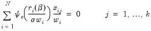 | (33.5) |
 , where
  , the derivative of the
  function, and
  is the value of the j-th regressor for observation
  .
. is not known, a sequential procedure is used that alternates between: (1) computing updated estimates of the scale
  given coefficient estimates
  , and (2) using iterative methods to find the
  that solves
Equation (33.5) for a given
that solves
Equation (33.5) for a given  . The initial
  are obtained from ordinary least squares. The initial coefficients are used to compute a scale estimate,
  , and from that are formed new coefficient estimates
  , followed by a new scale estimate
  , and so on until convergence is reached.
 , the updated scale
  is estimated using one of three different methods: Mean Absolute Deviation – Zero Centered (MADZERO), Median Absolute Deviation – Median Centered (MADMED), or Huber Scaling:
MADZERO | 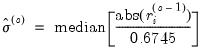 |
MADMED | 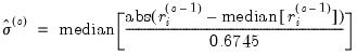 |
Huber | 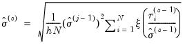 where 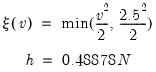 |
 are the residuals associated with
  and where the initial scale required for the Huber method is estimated by:
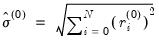 | (33.6) |
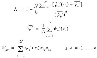
 statistic as
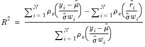
 is the M-estimate from the constant-only specification.
 is calculated as:
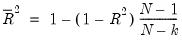 | (33.7) |
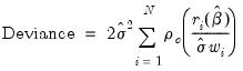
 statistic, and provide simulation results showing
  to be a better measure of fit than the robust
  outlined above. The
  statistic is defined as
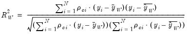 | (33.8) |
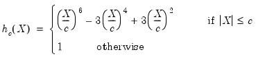
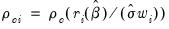 is the function of the residual value and
 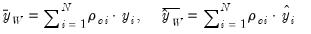 | (33.9) |
 , an adjusted value of
  may be calculated from the unadjusted statistic
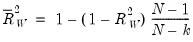 | (33.10) |
 statistic is a robust version of a Wald test of the hypothesis that all of the coefficients are equal to zero. It is calculated using the standard Wald test quadratic form:
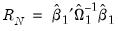 | (33.11) |
 are the
  non-intercept robust coefficient estimates and
  is the corresponding estimated covariance. Under the null hypothesis that all of the coefficients are equal to zero, the
  statistic is asymptotically distributed as a
  .
. | (33.12) |
 ), and a corresponding robust Schwarz Information Criterion (
 ):
):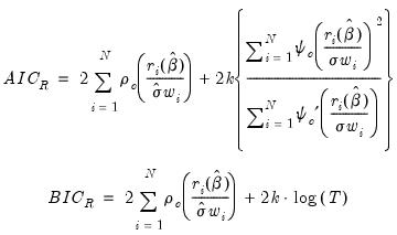 | (33.13) |
 is the derivative of
  as outlined in Holland and Welsch (1977). See Ronchetti (1985) for details.
 that provide the smallest estimate of the scale
  such that:
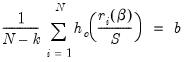 | (33.14) |
 with tuning constant
  , where
  is taken to be
  with
with  the standard normal. The breakdown value
  for this estimator is
 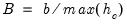 .
. | (33.15) |
 using the Median Absolute Deviation, Zero Centered (MADZERO) method.
 affects the objective function through
  and
and  .
.  is typically chosen to achieve a desired breakdown value. EViews defaults to a
  value of 1.5476 implying a breakdown value of 0.5. Other notable values for
  (with associated
  ) are:
  |  |
5.1824 | 0.10 |
4.0963 | 0.15 |
3.4207 | 0.20 |
2.9370 | 0.25 |
2.5608 | 0.30 |
1.9880 | 0.40 |
1.5476 | 0.50 |
 from the data and compute the least squares regression to obtain a
  . By default
  is set equal to
  , the number of regressors. (Note that with the default
  , the regression will produce an exact fit for the subsample.)
 refinements to the initial coefficient estimates using a variant of M-estimation which takes a single step toward the solution of
Equation (33.5) at every
refinements to the initial coefficient estimates using a variant of M-estimation which takes a single step toward the solution of
Equation (33.5) at every  update. These modified M-estimate refinements employ the Bisquare function
  with tuning parameter and scale estimator
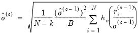 | (33.16) |
 is the previous iteration's estimate of the scale and
  is the breakdown value defined earlier.
 is obtained using MADZERO
 using MADZERO, and produce a final estimate of
  by iterating
Equation (33.16) (with
by iterating
Equation (33.16) (with  in place of
  ) to convergence or until
  .
.  times. The best (smallest)
  scale estimates are refined using M-estimation as in Step 2 with
  (or until convergence). The smallest scale from those refined scales is the final estimate of
  , and the final coefficient estimates are the corresponding estimates of
  .
. for S-estimation is given by:
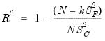 | (33.17) |
 is the estimate of the scale from the final estimation, and
  is an estimate of the scale from S-estimation with only a constant as a regressor.
 | (33.18) |
 statistic is identical to the one computed for M-estimation. See
“Rn-squared Statistic” for discussion.
statistic is identical to the one computed for M-estimation. See
“Rn-squared Statistic” for discussion.Type I (default) | 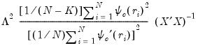 |
Type II | 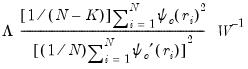 |
Type III | 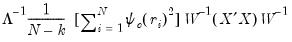 |
 | (33.19) |
 and
and  is the value of the j-th regressor for observation
  .
.