type=arg (default=“bk”) | Specify the type of band-pass filter: “bk” is the Baxter-King fixed length symmetric filter, “cffix” is the Christiano-Fitzgerald fixed length symmetric filter, “cfasym” is the Christiano-Fitzgerald full sample asymmetric filter. |
low=number, high=number | Low (  ) and high ( ) and high ( ) values for the cycle range to be passed through (specified in periods of the workfile frequency). ) values for the cycle range to be passed through (specified in periods of the workfile frequency). Defaults to the workfile equivalent corresponding to a range of 1.5–8 years for semi-annual to daily workfiles; otherwise sets “low=2”, “high=8”. The arguments must satisfy  . The corresponding frequency range to be passed through will be . The corresponding frequency range to be passed through will be 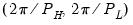 . . |
lag=integer | Fixed lag length (positive integer). Sets the fixed lead/lag length for fixed length filters (“type=bk” or “type=cffix”). Must be less than half the sample size. Defaults to the workfile equivalent of 3 years for semi-annual to daily workfiles; otherwise sets “lag=3”. |
iorder=[0,1] (default=0) | Specifies the integration order of the series. The default value, “0” implies that the series is assumed to be (covariance) stationary; “1” implies that the series contains a unit root. The integration order is only used in the computation of Christiano-Fitzgerald filter weights (“type=cffix” or “type=cfasym”). When “iorder=1”, the filter weights are constrained to sum to zero. |
detrend=arg (default=“n”) | Detrending method for Christiano-Fitzgerald filters (“type=cffix” or “type=cfasym”). You may select the default argument “n” for no detrending, “c” to demean, or “t” to remove a constant and linear trend. You may use the argument “d” to remove drift, if the option “iorder=1” is also specified. |
nogain | Suppresses plotting of the frequency response (gain) function for fixed length symmetric filters (“type=bk” or “type=cffix”). By default, EViews will plot the gain function. |
noncyc=arg | Specifies a name for a series to contain the non-cyclical series (difference between the actual and the filtered series). If no name is provided, the non-cyclical series will not be saved in the workfile. |
w=arg | Store the filter weights as an object with the specified name. For fixed length symmetric filters (“type=bk” or “type=cffix”), the saved object will be a matrix of dimension  where where  is the user-specified lag length order. For these filters, the weights on the leads and the lags are the same, so the returned matrix contains only the one-sided weights. The filtered series is the user-specified lag length order. For these filters, the weights on the leads and the lags are the same, so the returned matrix contains only the one-sided weights. The filtered series  may be computed as: may be computed as: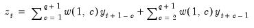 for 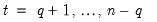 . .For time-varying filters, the weight matrix is of dimension  where where  is the number of non-missing observations in the current sample. Row is the number of non-missing observations in the current sample. Row  of the matrix contains the weighting vector used to generate the of the matrix contains the weighting vector used to generate the  -th observation of the filtered series, where column -th observation of the filtered series, where column  contains the weight on the contains the weight on the  -th observation of the original series. The filtered series may be computed as: -th observation of the original series. The filtered series may be computed as: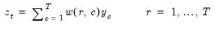 where  is the original series and is the original series and  is the is the  element of the weighting matrix. By construction, the first and last rows of the weight matrix will be filled with missing values for the symmetric filter. element of the weighting matrix. By construction, the first and last rows of the weight matrix will be filled with missing values for the symmetric filter. |
prompt | Force the dialog to appear from within a program. |
p | Print the graph. |