Background
The following discussion describes only the basic features of switching models. Switching models have a long history in economics that is detailed in numerous surveys (Goldfeld and Quandt, 1973, 1976; Maddala, 1986; Hamilton, 1994; Frühwirth-Schnatter, 2006), and we encourage you to explore these resources for additional discussion.
The Basic Model
Suppose that the random variable of interest,

follows a process that depends on the value of an unobserved discrete state variable

. We assume there are

possible regimes, and we are said to be in state or regime

in period

when

, for
.
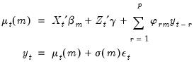
The switching model assumes that there is a different regression model associated with each regime. Given regressors

and

, the conditional mean of

in regime

is assumed to be the linear specification:
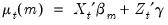 | (39.1) |
where

and

are

and

vectors of coefficients. Note that the

coefficients for

are indexed by regime and that the

coefficients associated with

are regime invariant.
Lastly, we assume that the regression errors are normally distributed with variance that may depend on the regime. Then we have the model:
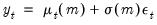 | (39.2) |
when

, where

is

standard normally distributed. Note that the standard deviation

may be regime dependent,

.
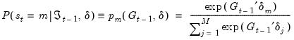
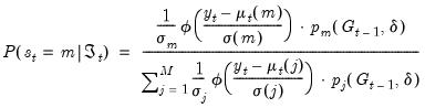
The likelihood contribution for a given observation may be formed by weighting the density function in each of the regimes by the one-step ahead probability of being in that regime:
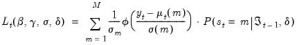 | (39.3) |
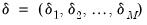
,
,

are parameters that determine the regime probabilities,

is the standard normal density function, and

is the information set in period

. In the simplest case, the

represent the regime probabilities themselves.
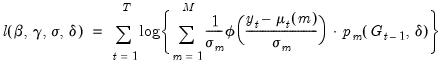
The full log-likelihood is a normal mixture
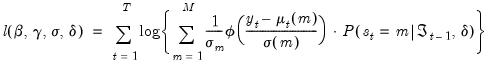 | (39.4) |
which may be maximized with respect to

.
Simple Switching
To this point, we have treated the regime probabilities
in an abstract fashion. This section considers a simple switching model featuring independent regime probabilities. We begin by focusing on the specification of the regime probabilities, then describe likelihood evaluation and estimation of those probabilities.
It should be emphasized that the following discussion is valid only for specifications with uncorrelated errors. Models with correlated errors are described in
“Serial Correlation”.
Regime Probabilities
In the case where the probabilities are constant values, we could simply treat them as additional parameters in the likelihood in
Equation (39.4). More generally, we may allow for varying probabilities by assuming that

is a function of vectors of exogenous observables

and coefficients

parameterized using a multinomial logit specification:
 | (39.5) |
for
with the identifying normalization

. The special case of constant probabilities is handled by choosing

to be identically equal to 1.
Likelihood Evaluation
We may use
Equation (39.4) and
Equation (39.5) to obtain a normal mixture log-likelihood function:
 | (39.6) |
This likelihood may be maximized with respect to the parameters

using iterative methods.
It is worth noting that the likelihood function for this normal mixture model is unbounded for certain parameter values. However, local optima have the usual consistency, asymptotic normality, and efficiency properties. See Maddala (1986) for discussion of this issue as well as a survey of different algorithms and approaches for estimating the parameters.
Given parameter point-estimates, coefficient covariances may be estimated using conventional methods, e.g., inverse negative Hessian, inverse outer-product of the scores, and robust sandwich.
Filtering
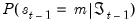
The likelihood expression in
Equation (39.6) depends on the one-step ahead probabilities of being in a regime:
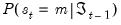
. Note, however, that observing the value of the dependent variable in a given period provides additional information about which regime is in effect. We may use this contemporaneous information to obtain updated estimates of the regime probabilities
The process by which the probability estimates are updated is commonly termed filtering. By Bayes’ theorem and the laws of conditional probability, we have the filtering expressions:
 | (39.7) |
The expressions on the right-hand side are obtained as a by-product of the densities obtained during likelihood evaluation. Substituting, we have:
 | (39.8) |
Markov Switching
The Markov switching regression model extends the simple exogenous probability framework by specifying a first-order Markov process for the regime probabilities. We begin by describing the regime probability specification, then discuss likelihood computation, filtering, and smoothing.
Regime Probabilities
The first-order Markov assumption requires that the probability of being in a regime depends on the previous state, so that
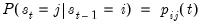 | (39.9) |
Typically, these probabilities are assumed to be time-invariant so that

for all

, but this restriction is not required.
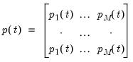
We may write these probabilities in a transition matrix
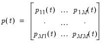 | (39.10) |
where the

-th element represents the probability of transitioning from regime

in period

to regime

in period

. (Note that some authors use the transpose of

so that all of their indices are reversed from those used here.)
As in the simple switching model, we may parameterize the probabilities in terms of a multinomial logit. Note that since each row of the transition matrix specifies a full set of conditional probabilities, we define a separate multinomial specification for each row

of the matrix
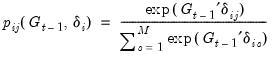 | (39.11) |
for

and

with the normalizations

.
As noted earlier, Markov switching models are generally specified with constant probabilities so that

contains only a constant. Hamilton’s (1989) model of GDP is a notable example of a constant transition probability specification. Alternately, Diebold, Lee, and Weinbach (1994), and Filardo (1994) adopt two-state models that employ time-varying logistic parameterized probabilities.
Likelihood Evaluation and Filtering
The Markov property of the transition probabilities implies that the expressions on the right-hand side of
Equation (39.4) must be evaluated recursively.
Briefly, each recursion step begins with filtered estimates of the regime probabilities for the previous period. Given filtered probabilities,
, the recursion may broken down into three steps:
1. We first form the one-step ahead predictions of the regime probabilities using basic rules of probability and the Markov transition matrix:
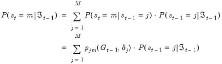 | (39.12) |
2. Next, we use these one-step ahead probabilities to form the one-step ahead joint densities of the data and regimes in period

:
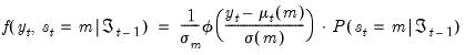 | (39.13) |
3. The likelihood contribution for period

is obtained by summing the joint probabilities across unobserved states to obtain the marginal distribution of the observed data
 | (39.14) |
4. The final step is to filter the probabilities by using the results in
Equation (39.13) to update one-step ahead predictions of the probabilities:
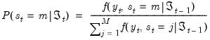 | (39.15) |
These steps are repeated successively for each period,

. All that we require for implementation are the initial filtered probabilities,

, or alternately, the initial one-step ahead regime probabilities
. See
“Initial Probabilities” for discussion.
The likelihood obtained by summing the terms in
Equation (39.14) may be maximized with respect to the parameters

using iterative methods. Coefficient covariances may be estimated using standard approaches.
Smoothing
Estimates of the regime probabilities may be improved by using all of the information in the sample. The
smoothed estimates for the regime probabilities in period

use the information set in the final period,

, in contrast to the filtered estimates which employ only contemporaneous information,

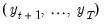
. Intuitively, using information about future realizations of the dependent variable

(

) improves our estimates of being in regime

in period

because the Markov transition probabilities link together the likelihood of the observed data in different periods.
Kim (2004) provides an efficient smoothing algorithm that requires only a single backward recursion through the data. Under the Markov assumption, Kim shows that the joint probability is given by
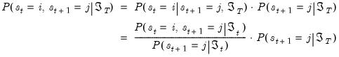 | (39.16) |
The key in moving from the first to the second line of
Equation (39.16) is the fact that under appropriate assumptions, if

were known, there is no additional information about

in the future data
.
The smoothed probability in period

is then obtained by marginalizing the joint probability with respect to

:
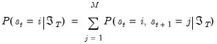 | (39.17) |
Note that apart from the smoothed probability terms,
, all of the terms on the right-hand side of
Equation (39.16) are obtained as part of the filtering computations. Given the set of filtered probabilities, we initialize the smoother using
, and iterate computation of
Equation (39.16) and
Equation (39.17) for
to obtain the smoothed values.
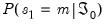
Initial Probabilities
The Markov switching filter requires initialization of the filtered regime probabilities in period 0,
.
There are a few ways to proceed. Most commonly, the initial regime probabilities are set to the ergodic (steady state) values implied by the Markov transition matrix (see, for example Hamilton (1999, p. 192) or Kim and Nelson (1999, p. 70) for discussion and results). The values are thus treated as functions of the parameters that determine the transition matrix.
Alternately, we may use prior knowledge to specify regime probability values, or we can be agnostic and assign equal probabilities to regimes. Lastly, we may treat the initial probabilities as parameters to be estimated.
Note that the initialization to ergodic values using period 0 information is somewhat arbitrary in the case of time-varying transition probabilities.
Dynamic Models
We may extend the basic switching model to allow for dynamics in the form of lagged endogenous variables and serially correlated errors. The two methods require different assumptions about the dynamic response to changes in regime.
Our discussion is very brief. Frühwirth-Schnatter (2006) offers a nice overview of the differences between these two approaches, and provides further discussion and references.
Dynamic Regression
The most straightforward method of adding dynamics to the switching model is to include lagged endogenous variables. For a model with

lagged endogenous regressors, and random state variable

taking the value

we have:
 | (39.18) |
where

is again

standard normally distributed. The coefficients on the lagged endogenous variable are allowed to be regime-varying, but this generality is not required.
In the Markov switching context, this model has been termed the “Markov switching dynamic regression” (MSDR) model (Frühwirth-Schnatter, 2006). In the special case where the lagged endogenous coefficients are regime-invariant, the model may be viewed as a variant of the “Markov switching intercept” (MSI) specification (Krolzig, 1997).
Of central importance is the fact that the mean specification depends only on the contemporaneous state variable

so that lagged endogenous regressors may be treated as additional regime specific

or invariant

for purposes of likelihood evaluation, filtering, and smoothing. Thus, the discussions in
“Simple Switching” and
“Markov Switching” are directly applicable in MSDR settings.
Serial Correlation
An alternative dynamic approach assumes that the errors are serially correlated (Hamilton, 1989). With serial correlation of order

, we have the AR specification
 | (39.19) |
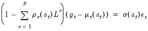
Rearranging terms and applying the lag operator, we have:
 | (39.20) |
In the Markov switching literature, this specification has been termed the “Markov switching autoregressive” (MSAR) (Frühwirth-Schnatter, 2006) or the “Markov switching mean” (MSM) model (Krolzig, 1997). The MSAR model is perhaps most commonly referred to as the “Hamilton model” of switching with dynamics.
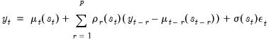
Note that, in contrast to the MSDR specification, the mean equation in the MSAR model depends on lag states. The presence of the regime-specific lagged mean adjustments on the right-hand side of
Equation (39.20) implies that probabilities for a

dimensional state vector representing the current and

previous regimes are required to obtain a representation of the likelihood.
For example, in a two regime model with an AR(1), we have the standard prediction error representation of the likelihood:
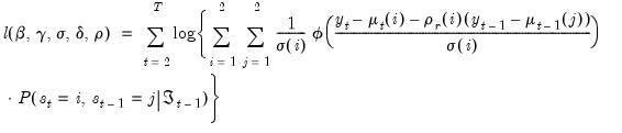 | (39.21) |
which requires that we consider probabilities for the four potential regime outcomes for the state vector

.
More generally, since there is a

dimensional state vector and

regimes, the number of potential realizations is

. The description of the basic Markov switching model above (
“Markov Switching”) is no longer valid since it does not handle the filtering and smoothing for the full

vector of probabilities.
Markov Switching AR
Hamilton (1989) derived the form of the MSAR specification and outlined an operational filtering procedure for evaluating the likelihood function. Hamilton (1989), Kim (1994), and Kim and Nelson (1999, Chapter 4) all offer excellent descriptions of the construction of this lagged-state filtering procedure.
Briefly, the Hamilton filter extends the analysis in
“Markov Switching” to handle the larger

dimensional state vector. While the mechanics of the procedure are a bit more involved, the concepts follow directly from the simple filter described above (
“Likelihood Evaluation and Filtering”). The filtered probabilities for lagged values of the states,
conditional on the information set

are obtained from the previous iteration of the filter, and the one-step ahead joint probabilities for the state vector are obtained by applying the Markov updates to the filtered probabilities. These joint probabilities are used to evaluate a likelihood contribution and in obtaining updated filtered probabilities.
Hamilton also offers a modified lag-state smoothing algorithm that may be used with the MSAR model, but the approach is computationally unwieldy. Kim (1994) improves significantly on the Hamilton smoother with an efficient smoothing filter that handles the

probabilities using a single backward recursion pass through the data. This approach is a straightforward extension of the basic Kim smoother (see
“Smoothing”).
Simple Switching AR
The simple switching results outlined earlier (
“Simple Switching”) do not hold for the simple switching with autocorrelation (SSAR) model. As with the MSAR specification, the presence of lagged states in the specification complicates the dynamics and requires handling a

dimensional state variable representing current and lag states.
Conveniently, we may obtain results for the specification by treating it as a restricted Markov switching model with transition probabilities that do not depend on the origin regime:
 | (39.22) |
so that the rows of the transition matrix are the identical
 | (39.23) |
We may then apply the Hamilton filter and Kim smoother to this restricted specification to obtain the one-step ahead, likelihood, filtered, and smoothed values.
Initial Probabilities
In the serial correlation setting, the Markov switching filter requires initialization of the vector of probabilities associated with the

dimensional state vector. We may proceed as in the uncorrelated model by setting

initial probabilities in period

using one of the methods described in
“Initial Probabilities” and recursively applying Markov transition updates to obtain the joint initial probabilities for the

dimensional initial probability vector in period

.
Again note that the initialization to steady state values using the period

information is somewhat arbitrary in the case of time-varying transition probabilities.