To illustrate switching VAR estimation, we consider examples using quarterly GDP data for a subset of G7 countries obtained from the OECD National Accounts Statistics ( https://data.oecd.org/gdp/quarterly-gdp.htm).

We first estimate a Markov switching intercept model with varying intercepts, and then a Markov switching mean model with regime specific intercepts and lagged endogenous.

The data for this example consists of 1960q4–2018q4 quarterly percent change in GDP for Canada (DPCAN), Germany (DPDEU), Japan (DPJPN), and the US (DPUSA). The data may be found in the workfile “msvar_G7.WF1”.

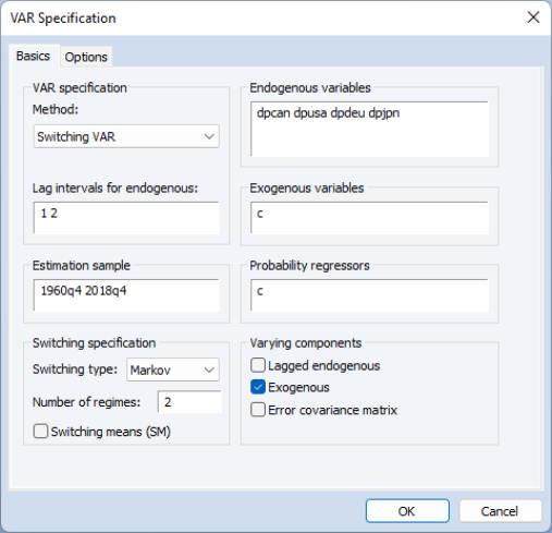
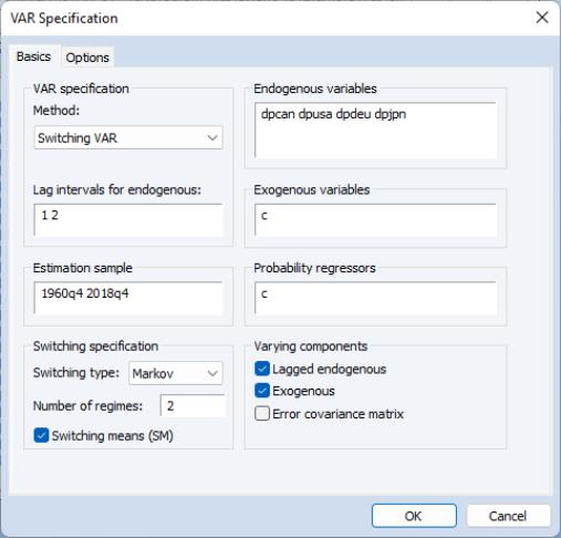
To estimate the first model, open the switching VAR dialog and enter the specification as depicted below:

The specification consists of a two-state Markov switching intercept VAR(2) with a single switching mean regressor C. The error variance is assumed to be common across the regimes. Adopting the general Krolzig (1997) taxonomy, we may term this an MSI-VAR(2) specification—Markov switching intercept, VAR(2). The only probability regressor is the constant C since we have time-invariant regime transition probabilities.

With the exception of the convergence tolerance which we set to 1e-8, we leave the rest of the settings at their default values. Click on OK to estimate the equation and display the estimation results.

The top portion of the output describes the estimation settings:

(Bear in mind that if you attempt replicate this estimation using the default settings, you may obtain different results due to the different set of random starting values. You may use the random number generator seed settings to obtain the same starting values.)

The middle section displays the coefficients for the regime specific mean and the invariant error distribution coefficients with columns corresponding to endogenous variables. We see, in the differences in the regime specific means, corresponding to fast and slow growth rates:

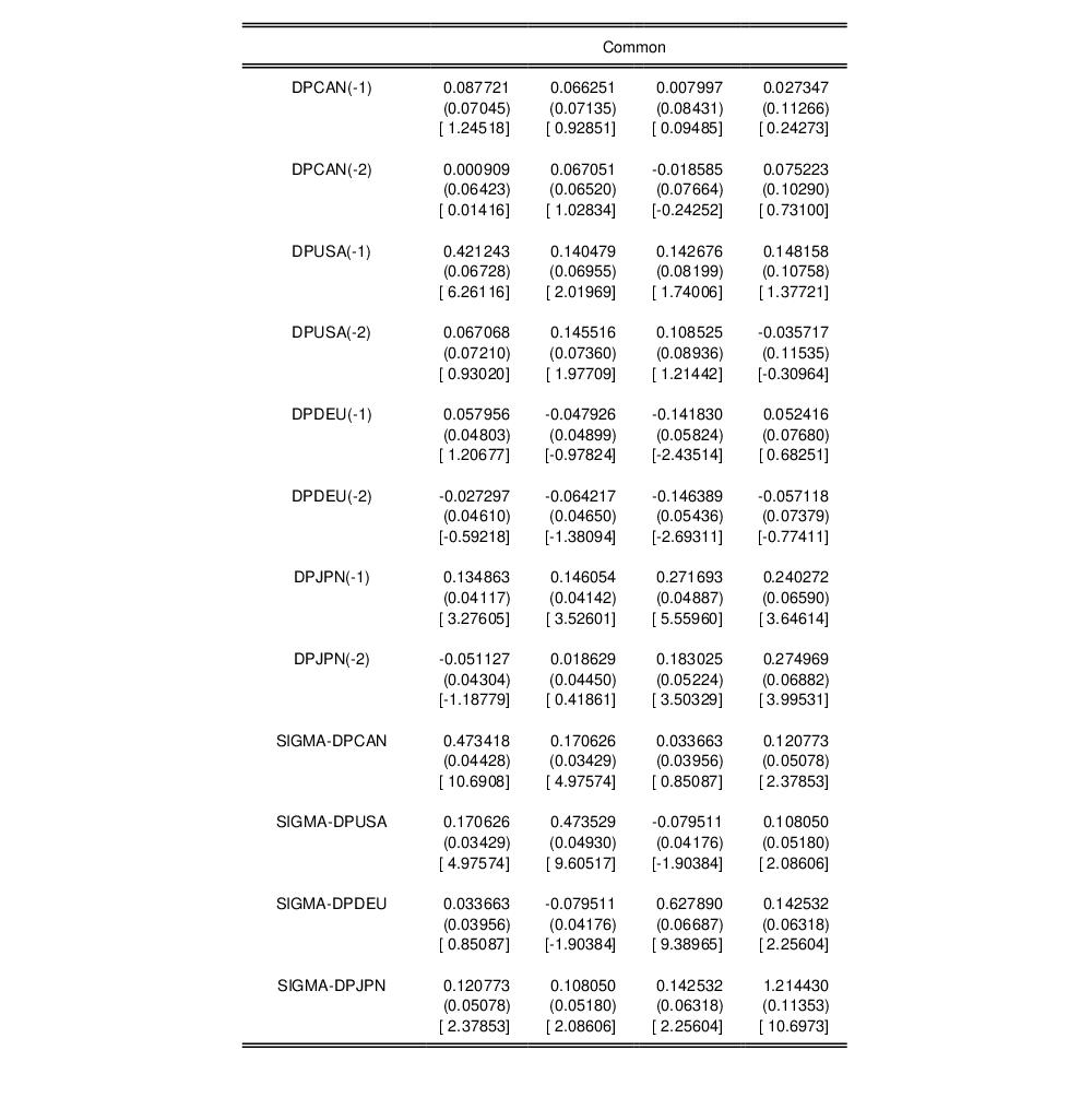
Next are the regime invariant (common) VAR lag coefficients and error covariance matrix:

The remaining results show the parameters of the transition matrix and summary statistics for the estimated VAR.

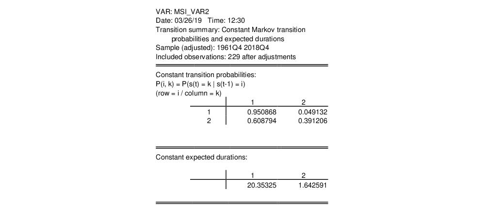
Instead of focusing on the transition matrix parameters, we examine the transition matrix probabilities directly by selecting View/Regime Results/Transition Results... and clicking on OK to display the default summary view:

Here, we see the transition probability matrix and the expected durations. Note that there is considerable state dependence in the transition probabilities with a higher probability of remaining in the high growth regime (0.95), but less so for the low growth regime (0.39). The corresponding expected durations in a regime are approximately 10.4 and 4.1 quarters, respectively.

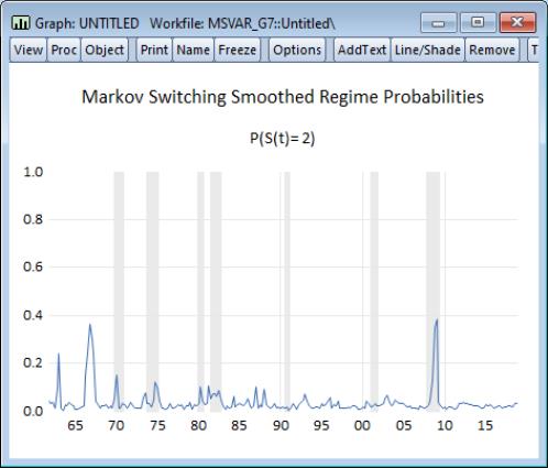
Lastly, we display the filtered and full sample estimates of the probabilities of being in the two regimes. First select View/Regime Results/Regime Probabilities... and choose the smoothed results. We will display the results only for the second regime.

After saving the view as a graph and applying the RecShade add-in,

to label the NBER recessions, we see that the predicted probabilities of being in the low output state generally coincide with the commonly employed definition of US recessions:

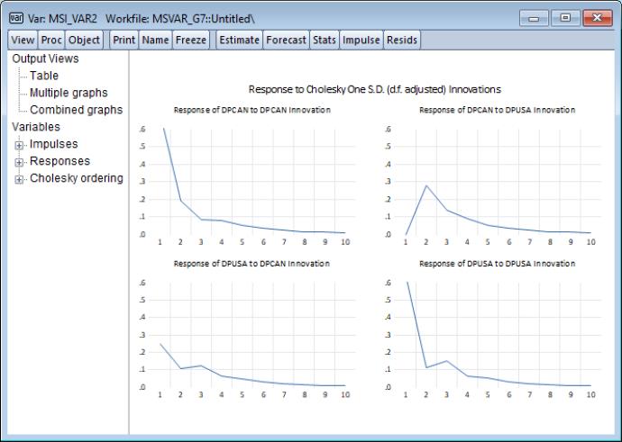
We may examine the impulse responses for this VAR in the usual fashion. Click on View/Impulse Response... edit the fields to show the impulses and responses for the first two endogenous variables, and click on OK to display the results:

We may estimate a two-state Markov switching mean VAR(2) with switching mean regressor C, switching VAR lag coefficients. and common error variance (MSMA-VAR(2)).

We leave the remaining settings at their defaults and click on OK to estimate the equation. Following estimation, EViews displays the results.

First, the top portion shows the specification settings:

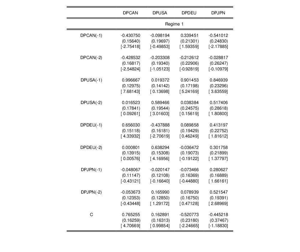
The next section contains results for the regime varying results; first for regime 1,

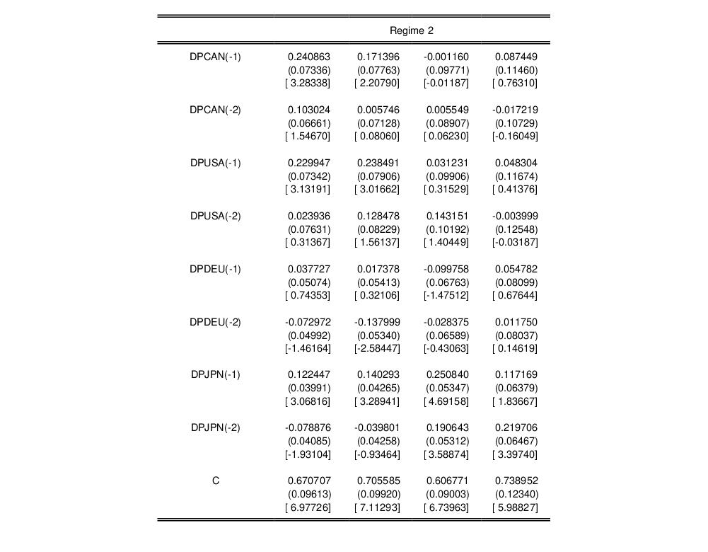
and then for regime 2,

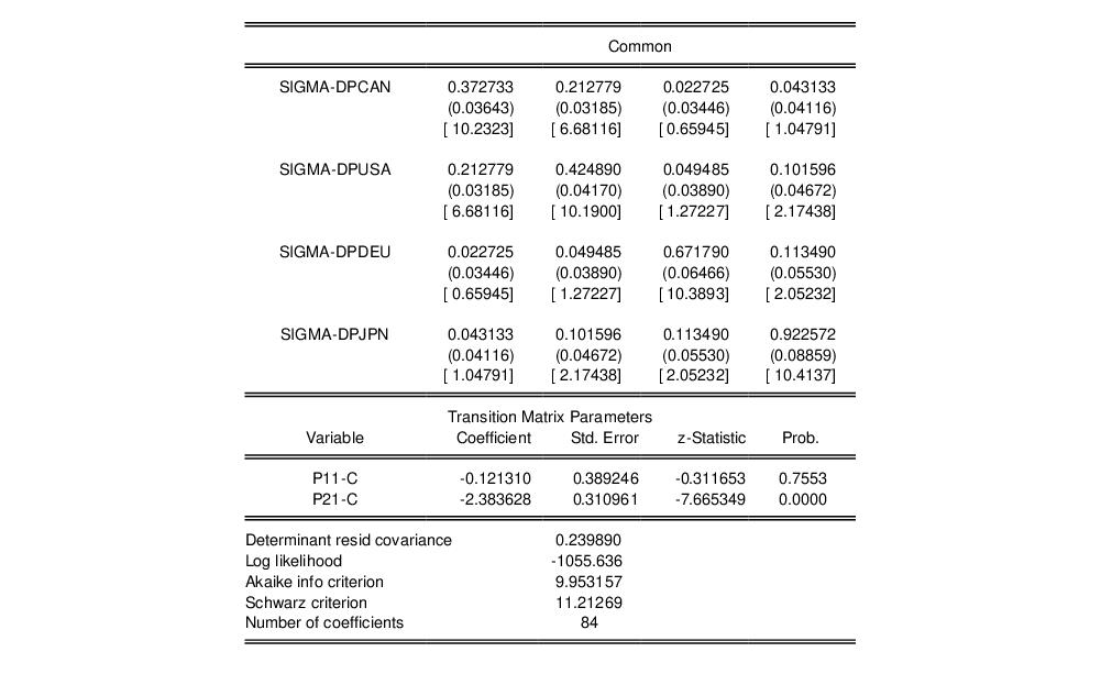
and then the common coefficients and summary statistics

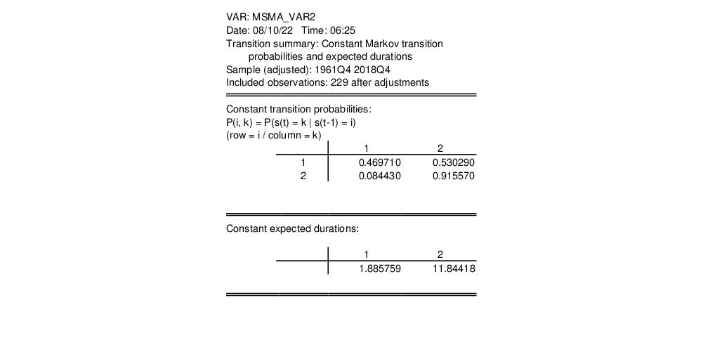
We can examine directly the transition probabilities. The default transition probability summary (View/Regime Results/Transition Results...) shows descriptive statistics for the elements of the transition matrix:

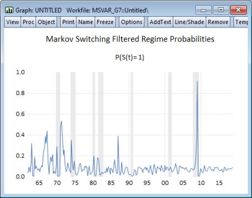
The filtered probabilities of being in the regime 1, with NBER recession shading are:

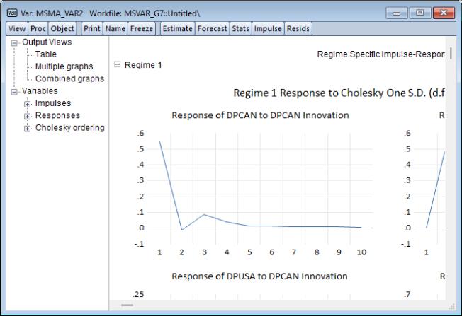
Examining the impulse responses, we click on View/Impulse Response... edit the fields to show the impulses and responses for the first two endogenous variables, and click on OK to display the results:

Notice that the results are displayed in a spool, with impulse responses computed for each set of regime-specific coefficients.