Equation Diagnostics
In addition to the usual views and procs for an equation such as coefficient confidence ellipses, Wald tests, omitted and redundant variables tests, EViews offers diagnostics for examining the properties of your ARMA model and the properties of the estimated innovations.
ARMA Structure
This set of views provides access to several diagnostic views that help you assess the structure of the ARMA portion of the estimated equation. The view is currently available only for models specified by list that includes at least one AR or MA term and estimated by least squares. There are three views available: roots, correlogram, and impulse response.
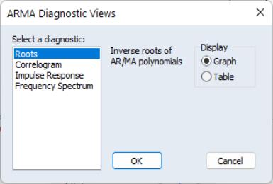
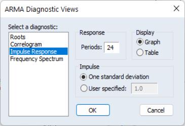
To display the ARMA structure, select from the menu of an estimated equation. If the equation type supports this view and there are no ARMA components in the specification, EViews will open the dialog:
On the left-hand side of the dialog, you will select one of the three types of diagnostics. When you click on one of the types, the right-hand side of the dialog will change to show you the options for each type.
Roots
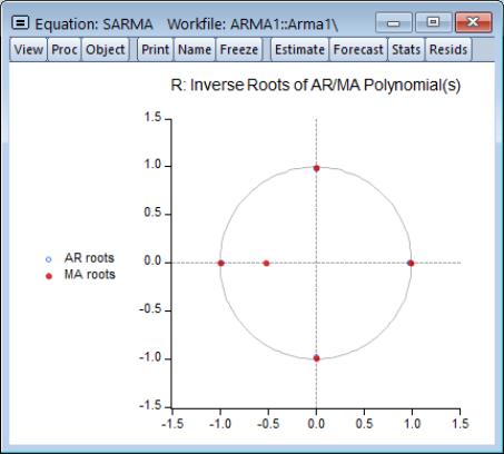
The roots view displays the inverse roots of the AR and/or MA characteristic polynomial. The roots may be displayed as a graph or as a table by selecting the appropriate radio button.
The graph view plots the roots in the complex plane where the horizontal axis is the real part and the vertical axis is the imaginary part of each root.
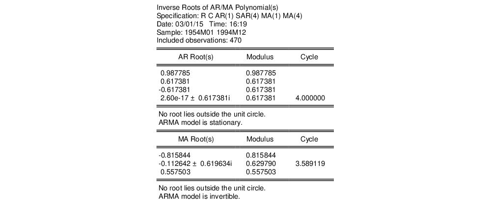
If the estimated ARMA process is (covariance) stationary, then all AR roots should lie inside the unit circle. If the estimated ARMA process is invertible, then all MA roots should lie inside the unit circle. The table view displays all roots in order of decreasing modulus (square root of the sum of squares of the real and imaginary parts).
For imaginary roots (which come in conjugate pairs), we also display the cycle corresponding to that root. The cycle is computed as

, where
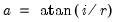
, and

and

are the imaginary and real parts of the root, respectively. The cycle for a real root is infinite and is not reported.
Correlogram
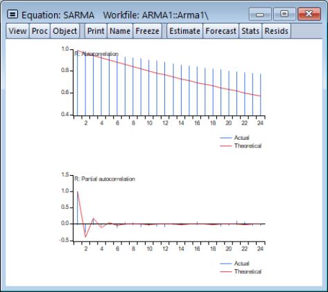
The correlogram view compares the autocorrelation pattern of the structural residuals and that of the estimated model for a specified number of periods (recall that the structural residuals are the residuals after removing the effect of the fitted exogenous regressors but not the ARMA terms). For a properly specified model, the residual and theoretical (estimated) autocorrelations and partial autocorrelations should be “close”.
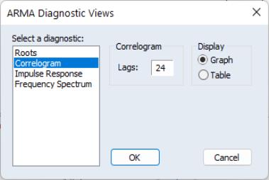
To perform the comparison, simply select the diagnostic, specify a number of lags to be evaluated, and a display format ( or ).
Here, we have specified a graphical comparison over 24 periods/lags. The graph view plots the autocorrelations and partial autocorrelations of the sample structural residuals and those that are implied from the estimated ARMA parameters. If the estimated ARMA model is not stationary, only the sample second moments from the structural residuals are plotted.
The table view displays the numerical values for each of the second moments and the difference between from the estimated theoretical. If the estimated ARMA model is not stationary, the theoretical second moments implied from the estimated ARMA parameters will be filled with NAs.
Note that the table view starts from lag zero, while the graph view starts from lag one.
Impulse Response
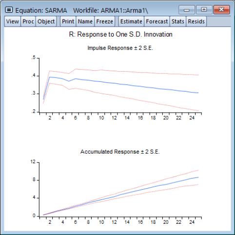
The ARMA impulse response view traces the response of the ARMA part of the estimated equation to shocks in the innovation.
An impulse response function traces the response to a one-time shock in the innovation. The accumulated response is the accumulated sum of the impulse responses. It can be interpreted as the response to step impulse where the same shock occurs in every period from the first.
To compute the impulse response (and accumulated responses), select the diagnostic, enter the number of periods, and display type, and define the shock. For the latter, you have the choice of using a one standard deviation shock (using the standard error of the regression for the estimated equation), or providing a user specified value. Note that if you select a one standard deviation shock, EViews will take account of innovation uncertainty when estimating the standard errors of the responses.
If the estimated ARMA model is stationary, the impulse responses will asymptote to zero, while the accumulated responses will asymptote to its long-run value. These asymptotic values will be shown as dotted horizontal lines in the graph view.
For a highly persistent near unit root but stationary process, the asymptotes may not be drawn in the graph for a short horizon. For a table view, the asymptotic values (together with its standard errors) will be shown at the bottom of the table. If the estimated ARMA process is not stationary, the asymptotic values will not be displayed since they do not exist.
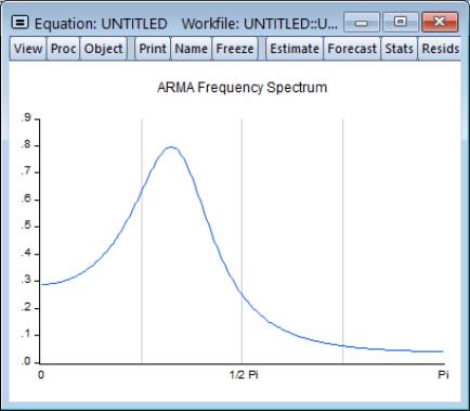
ARMA Frequency Spectrum
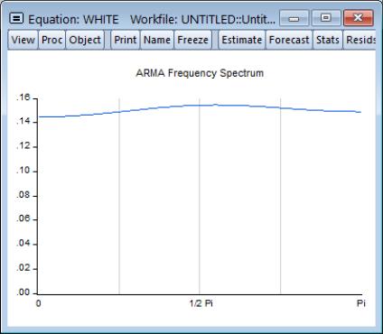
The ARMA frequency spectrum view of an ARMA equation shows the spectrum of the estimated ARMA terms in the frequency domain, rather than the typical time domain. Whereas viewing the ARMA terms in the time domain lets you view the autocorrelation functions of the data, viewing them in the frequency domain lets you observe more complicated cyclical characteristics.
The spectrum of an ARMA process can be written as a function of its frequency,

, where

is measured in radians, and thus takes values from

to

. However since the spectrum is symmetric around 0, it is EViews displays it in the range

.
To show the frequency spectrum, select from the equation toolbar, choose from the list box, and then select a display format ( or ).
If a series is white noise, the frequency spectrum should be flat, that is a horizontal line. Here we display the graph of a series generated as random normals, and indeed, the graph is approximately a flat line.
If a series has strong AR components, the shape of the frequency spectrum will contain peaks at points of high cyclical frequencies. Here we show a typical AR(2) model, where the data were generated such that

and

.
Q-statistics
If your ARMA model is correctly specified, the residuals from the model should be nearly white noise. This means that there should be no serial correlation left in the residuals. The Durbin-Watson statistic reported in the regression output is a test for AR(1) in the absence of lagged dependent variables on the right-hand side. As discussed in
“Correlograms and Q-statistics”, more general tests for serial correlation in the residuals may be carried out with and .
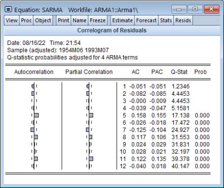
For the example seasonal ARMA model, the 12-period residual correlogram looks as follows:
The correlogram has a significant spike at lag 5, and all subsequent Q-statistics are highly significant. This result clearly indicates the need for respecification of the model.