Background
Cointegration
An understanding of VECMs requires a discussion of the notion of system-wide integration and equilibrium. Some important definitions will set the stage for our discussion:
• An individual time series

is said to be integrated of order

,

, if

is stationary, or

, while

is non-stationary.
• A system of

time series

is said to be integrated of order

,

, if at least one of its constituent series

is

, and no series is

for

. Note that this definition does not preclude a subset of the system series from being of lower order (or even stationary).
• An

system is said to be cointegrated if a linear combination of the constituent series is integrated of (lower) order,

where

. Further, a system

that is integrated of order

is said to be cointegrated of order

if there exists a cointegrating

-vector

such that

. Notice that

is not unique since multiplication by any nonzero constant yields a different cointegrating vector.
To simplify the following discussion, we will, without loss of generality, restrict

to 1 and

to 0 so that

and

.
The concept of cointegration introduced above is closely related to the notion of economic equilibrium. While individual economic processes may have volatile paths of evolution, there may be global forces which eventually produce stable paths of evolution. In particular, a group of economic variables may individually be

, or non-stationary, but there may exist cointegrated processes (linear combinations) which are

, or stationary. In this case, the cointegrated process is mean-reverting so that it while it may deviate from its expected value in the short-run, it eventually settles at its long-run (asymptotic) expected value.
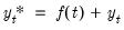
The VECM Specification
When

, the traditional levels-form VAR process is not the most useful representation since both the number and explicit form of any cointegrating relations are not easily obtained from this specification. Consequently, when analyzing cointegrating relationships we typically work with the VECM representation of the process.
The Basic VECM
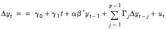
Consider a VAR process of order

:
 | (45.1) |
where
is a

-vector of endogenous variables,

are

matrices of coefficients, and the residual vector
is distributed with mean 0 and variance matrix

. Note that for simplicity, we assume that there are no deterministic terms in the VAR. This restriction is relaxed in the discussion of
“VECMs with Deterministics”.
The stability of the system is determined by the solutions to the determinant of the characteristic polynomial,
 | (45.2) |
The process is said to be stable if the roots of the polynomial lie outside the complex unit circle, or have modulus greater than 1.
Note that when at least one constituent series

is

, the VAR process is
unstable since we may show that
 | (45.3) |
is singular,

, and
Equation (45.2) is satisfied for roots lying on the unit circle.
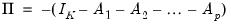
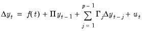
In general,

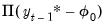
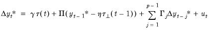
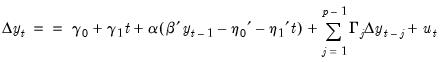
plays a key role in identifying both the number and nature of any cointegrating relationships. To better understand this role, we subtract

from both sides of the VAR representation
Equation (45.1) and rearrange terms to obtain the VECM representation:
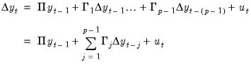 | (45.4) |
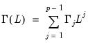
where
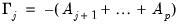 | (45.5) |
for

.
To obtain this representation, we first take the VAR representation and subtract off the lag of the endogenous variables from both sides:
 | (45.6) |
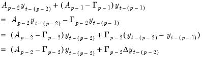
Next, we reparameterize the model by rewriting the remaining elements of the right-hand side as differences. Rewriting with the last two elements of the expression, we have
where
 | (45.7) |
Similarly, we may transform the last two non-difference terms in this new expression. Focusing on just those two terms, we have
 | (45.8) |
Define
 | (45.9) |
Then we may rewrite the

term as a difference using
 | (45.10) |
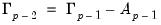
Notice that this process of rewriting the last two non-difference terms forms a recursion. For the remaining non-difference pairs, we may write,
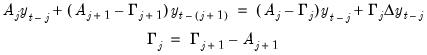 | (45.11) |
for
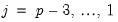
. Substituting recursion
Equation (45.11) into
Equation (45.6), we have:
 | (45.12) |
Then, using the initial value

from
Equation (45.7) and the recursion
Equation (45.9), we have
 | (45.13) |
Note that we may recover the parameters of the VAR from the parameters of the VECM using the relations
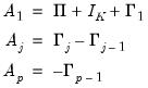 | (45.14) |
for

.
To see the central role of

in cointegration analysis, we focus on

, the matrix rank of

, where

.
Since our discussion assumes that

is

, it follows that

, and the

are

for all

. There are two important implications of these conditions. First, since

, it follows that

has reduced rank (

). Second, since the

are all

, to balance the order of both sides of
Equation (45.4),

must also be

.
For any

, there exist

matrices

and

each of rank

, such that
 | (45.15) |
where

is the transpose operator. Then we may write
 | (45.16) |
and given our assumptions,

must be an

linear combination of the series in the system, with

representing the cointegrating rank, and

the

cointegrating matrix.

is typically referred to as the loading matrix.
Note that although

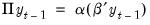
is not unique, a suitable normalization is possible by rearranging the variables so that the first

rows of the matrix are linearly independent:
 | (45.17) |
where

is a

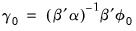
matrix. See Lütkepohl (2005) for details.
Lastly if

, balancing both sides of
Equation (45.6) requires

. In this case we say that there are no cointegrating relations since no linear combinations of

are

.
Basic VECM Estimation
While there are several methods for estimation of VECMs, we focus on the maximum likelihood (ML) variant, also known as reduced rank regression (RRR) (see Johansen (1995) and Lütkepohl (2005) for a detailed exposition).
Formally, RRR assumes a known cointegration rank

, Gaussian innovation vectors

, a time dimension of length

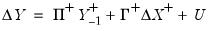
, and is best described using the VECM matrix representation (
Equation (45.4)):
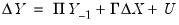 | (45.18) |
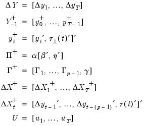
where
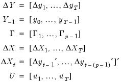 | (45.19) |
The RRR estimator is then the maximizer of the log-likelihood objective function:
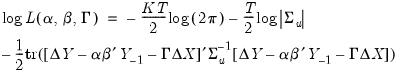 | (45.20) |
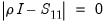
Johanson (1995) shows that optimizing the likelihood is equivalent to solving the eigenvalue problem
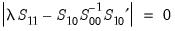 | (45.21) |
under the constraint
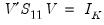
, where
are the

eigenvalues associated with eigenvector matrix
, and
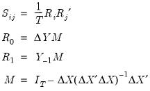 | (45.22) |
Solving the constrained eigenvalue problem yields

that are the eigenvalues of the symmetric matrix
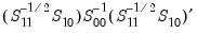 | (45.23) |
In terms of computation, note that

and

are the residuals from regression of the

and

on the

. Further,

may be obtained by first diagonalizing

using the solution to the auxiliary eigenvalue problem
 | (45.24) |
to obtain eigenvalues
and associated eigenvector matrix
. The square root of the inverse of

can then be estimated as
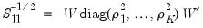 | (45.25) |
and the log-likelihood
Equation (45.20) is maximized at
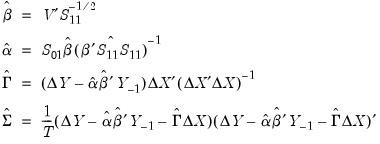 | (45.26) |
VECMs with Deterministics
The discussion thus far has ignored the presence of deterministic terms in the VAR specification. The inclusion of deterministics has important implications for the estimation and interpretation of VECMs, and there are different approaches to incorporating these terms.
The Classical Approach
Following Lütkepohl (2005), the classical approach to incorporating deterministic terms in VECMs is to let

follow a basic VAR(

) as in
Equation (45.1), and to work with the augmented process,
 | (45.27) |
where

denotes any

-dimensional deterministic function of time, often a low-order polynomial in

.
Substituting
into the VECM
Equation (45.4), we obtain:
 | (45.28) |
For example, if

is a constant function,

, then

for all

, and we have
 | (45.29) |
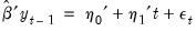
In this case, the constant function

may either be viewed as an intercept inside the cointegrating relation,
, or simply as an overall intercept

in the VECM. Importantly, in the latter case, the overall

is said to be
restricted since it must satisfy the restriction

imposed by the cointegrating relationship.
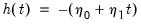
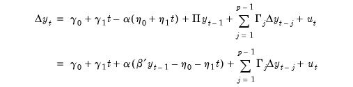
Likewise, if

is a linear trend,

, then

for all

, we have
 | (45.30) |
In this case, the trend function

may be included as a term in the cointegrating relation,
along with the
term appearing in the short-run dynamics, or as an overall intercept and trend in VECM (

). Notably, while the overall trend coefficient

is restricted by the cointegrating relationship, the constant

is
unrestricted as it contains free parameters unrelated to

from the short-run dynamics.
Lütkepohl (2005) emphasizes the importance of the cointegrating restrictions in governing the dynamic behavior of the levels of

, noting that their removal induces additional deterministics in the integrated VAR representation of the VECM. For example, if the restriction on

in
Equation (45.29) is removed, the corresponding integrated VAR specification will have a deterministic trend in the mean. Similarly, removing the restriction on

in
Equation (45.30) will generate a quadratic trend in the VAR.
We can make the separation between restricted and unrestricted deterministics concrete by re-parameterizing
Equation (45.28) to provide a general framework for a VECM with deterministics:
 | (45.31) |
where

and

are vector-valued functions denoting unrestricted and restricted deterministics, respectively, with corresponding coefficients

and

.

and

are assumed to be exclusive so that any deterministic function in

is not included in

, and vice versa. For the constant function

above,

is empty and

. For the linear trend function

,

, and

.
Lastly, note that while this discussion has focused on deterministic functions of time, the framework allows for the consideration of other types of exogenous variables which enter either the restricted cointegrating or the unrestricted transitory space.
The Johansen, Hendry, and Juselius Approach
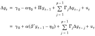
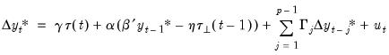
An alternative treatment of deterministics follows the conventions outlined in Johansen (1995), Hendry and Juselius (2001), and Juselius (2006), which we will term the JHJ approach. The approach begins with the VECM specification:
 | (45.32) |
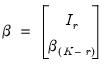
By virtue of cointegration, both

and

are stationary around their expected values. Taking expectations of
Equation (45.32) yields:
 | (45.33) |
for
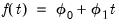
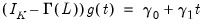
 | (45.34) |
where

is the lag operator.
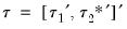
Let
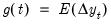
and
be the expected value paths of

and

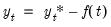
. Then rewriting
Equation (45.33) in terms of the deterministic component

yields,
 | (45.35) |
Johansen (1995) and Juselius (2006) show that

and

may be thought of as decompositions of

into components in the orthogonal directions of

and

. Since

is the weighting matrix for the expected congregating relation

,

are orthogonal weights for the expected common trends

(transitory variables).
It follows that this expression additively decomposes the deterministic function

into the space spanned by the transitory variables

, and the space spanned by the cointegrating relations

.
What distinguishes this decomposition from the classical approach is that each coefficient vector

can itself be decomposed into the spaces spanned by

and

. As discussed in Johansen (1995) and Juselius (2006), this result follows from a family of identities similar to
 | (45.36) |
Thus, each deterministic term can be decomposed into orthogonal components so that it appears simultaneously in the unrestricted (transitory) and restricted (cointegrated) spaces.
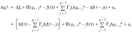
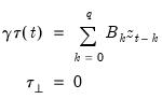
For example, when

is a constant function, we have the decomposition,
 | (45.37) |
 | (45.38) |
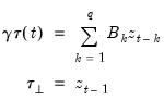
Similarly, when
is a linear trend function, the following decompositions follow:
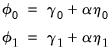 | (45.39) |
so that
and
. In this case the VECM in
Equation (45.32) is given by
 | (45.40) |
Estimating VECM with Deterministics
Estimation of VECMs with deterministics requires modification of the approach outlined in
“Basic VECM Estimation”.
Deterministic specifications which derive from the classical approach in
Equation (45.28) are accommodated by including the restricted deterministic regressors in the cointegrating space, and the unrestricted deterministics in the overall VECM. We modify
Equation (45.18) to provide:
 | (45.41) |
where
 | (45.42) |
where

and

,

and

are the unrestricted and restricted deterministic components and coefficients, respectively.
When deterministics are incorporated using the JHJ convention, the estimator must allow for the possibility that the same deterministic term can appear both inside the cointegrating equation and outside it.
It is useful to divide the cointegrating regressors and coefficients into those present only inside the cointegrating equation (

and

), those present only outside the equation (

and

), and those that are both inside and outside the cointegrating relation (

,

, and

) so that we have
and
, with coefficients

, and

.
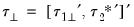
One estimation approach hinges on the ideas that the cointegrating (equilibrium) equation is stable around its mean of zero:
 | (45.43) |
Given this requirement, estimation may be conducted in three steps:
• Step 1: All dual deterministic regressors

are first removed from inside the cointegrating relationship, but retained outside. Then

,

and

are estimated using the classical approach outlined in
Equation (45.26) and
Equation (45.42) using deterministics

and coefficients

.
• Step 2: Given the estimates

and

from Step 1,

is estimated by choosing values of the coefficients so that the cointegrating equation has conditional mean zero:
 | (45.44) |
• Step 3: Using the estimates from Steps 1 and 2, the short-run coefficients

are estimated using appropriately modified versions of the expressions in
Equation (45.26) and
Equation (45.42) with deterministics

and coefficients

.
While there is no single approach for estimating the coefficients in Step 2 above, a simple linear regression of
on

satisfies the desired condition. When the deterministic regressors are the usual constant and trend, this regression reduces to a familiar least squares detrending of the cointegrating relation. See also Proposition 7.5 in Lütkepohl (2005). This is the method employed by EViews.
For example, consider a model where the constant and trend terms appear both inside and outside the cointegrating equation:
 | (45.45) |
• Step 1 estimates the classical model,
 | (45.46) |
to obtain estimates

and

, along with

,

, and

for
.
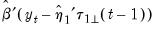
• Step 2 uses the least squares regression,
 | (45.47) |
to obtain estimates

and

.
• Step 3 updates the estimates of

,

, and the

using standard regression,
 | (45.48) |
The final coefficient estimates are given by

and

from Step 1,

and

from Step 2, and

from Step 3.
Popular VECM Deterministic Assumptions
The empirical literature has centered around five scenarios involving deterministic terms:
• Case 1: No deterministics, so that

,
in the classical framework, and
in the JHJ approach.
• Case 2: Restricted constant, so that

and

and

in the classical formulation, and

and

under JHJ.
Here, the constant is restricted to the cointegrating space and does not appear in the transitory space. The cointegrating mean is non-zero and the cointegrating equation restriction ensures that no linear trends exist in the corresponding VAR.
• Case 3: Unrestricted constant, so that

,

and

in the classical approach, and

and

for JHJ.
In this case, the constant appears in the transitory space but does not appear in the cointegrating space. The model has no deterministics in the cointegrating space, and exhibits a linear trend in the VAR representation.
• Case 3 (JHJ): Unrestricted constant in both the transitory and the cointegrating space so that
and
.
This JHJ model has a non-zero mean in the cointegrating relations, and has a linear trend in the corresponding VAR. Note that this case reduces to classical Case 3 when the restriction

is imposed.
• Case 4: Unrestricted constant and restricted trend so that

,

and

,

in the classical approach;

and

for

under JHJ.
Here, a constant appears in the transitory space but does not appear in the cointegrating space, and the trend term appears only in the cointegrating space. This model has a linear trend in the cointegrating relations, and has a linear trend in the corresponding VAR representation.
• Case 4 (JHJ): Unrestricted constant and restricted trend so that

and

in the JHJ framework.
The constant appears in both the transitory space and the cointegrating space, while the trend term appears only in the cointegrating space. The model has a non-zero mean and non-zero trend in the cointegrating relations, and has a linear trend in the corresponding VAR formulation. Note that this case reduces to classical Case 4 when the restriction

is imposed.
• Case 5: Unrestricted constant and trend, so that

,

and

in the classical approach;

,

and

under JHJ.
Here, the constant and trend appears in the transitory space. The model has a non-zero mean and non-zero trend in the cointegrating relations, and has a quadratic trend in the corresponding VAR.
• Case 5 (JHJ): Unrestricted constant and trend, so that
,

and
,

.
In this case, the constant and trend appear in both the transitory and cointegrating spaces. The model has a non-zero mean and non-zero trend in the cointegrating relations, and has a quadratic trend in the corresponding VAR formulation. Note that this case reduces to classical Case 5 when the restrictions

are imposed.
Exogenous Variables in VECMs
The endogenous variables

in our VEC model are the variables whose dynamics and evolution are determined within the VEC system. Given the autoregressive nature of the model, these variables are necessarily correlated with the errors

.
Accordingly, a particularly convenient (albeit slightly restrictive) definition of the exogenous variables in a VEC setting is any set of variables

which are independent of the error process

, and included in the VEC specification and estimated alongside their endogenous counterparts. Notice by this definition, deterministic regressors are examples of exogenous variables in VEC models.
The discussion on deterministics in
“Vector Error Correction Models (VECMs)” is applicable to arbitrary exogenous regressors, not just those which are deterministic regressors involving explicit polynomials of time. Thus incorporation of exogenous variables requires no meaningful adjustment to the estimation procedures outlined in
“Estimating VECM with Deterministics”.
More formally, let

denote a set of exogenous variables, and for generality, suppose we wish to include an order
q distributed lag of

in the VECM.
Starting with the classical convention for deterministics in
Equation (45.27), we specify a VAR(p) process where the endogenous variables are autoregressive of order p and whose difference specification includes exogenous variables that are distributed lag variables of order q. Then the exogenous component is assumed to be:
 | (45.49) |
where

are coefficient matrices associated with the lags of the exogenous variables.
Lütkepohl (2005) argues that the VEC representation of this model can assume two forms. In the first form, the endogenous variables

are cointegrated among themselves, but not with the set of exogenous variables

In this case, the VEC representation is given by:
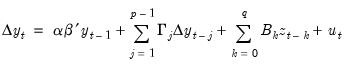 | (45.50) |
In the second form the endogenous variables are not only cointegrated among themselves, but also with the exogenous variables

. Here the VEC representation is:
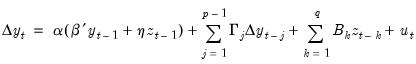 | (45.51) |
Notice that both of these specifications are embedded in the general classical framework for deterministics described above (
“The Classical Approach”):
 | (45.52) |
where in the first form, we have,
 | (45.53) |
while in the second form, we have,
 | (45.54) |
Similarly, it is possible to decompose each of the coefficient matrices

in (18) into the spaces spanned by

and

as in
“The Johansen, Hendry, and Juselius Approach”. This decomposition would produce a model in which exogenous regressors appear both among the long-run and short-run regressors.
While we see that exogenous regressors are conceptually analogous to deterministic regressors, caution must be exercised when augmenting VEC models with deterministic regressors. Notably, since the deterministic regressors enter into the differenced VEC models (
Equation (45.27) and
Equation (45.27)), their inclusion will have implications for the behavior of the equivalent VAR level form that should be considered. These nuances are analogous to role of deterministics in the unit root literature where, for instance, a constant term in a random walk will generate a linear trend in the mean. While these considerations are also present for the deterministic trend regressors, the implications for trend regressors are more obvious as the inclusion of the trends is generally described in terms of the effects on both the levels and the differences.

 and
and  . In other words,
 and the VECM in
Equation (45.32) may be written as:
and the VECM in
Equation (45.32) may be written as: