Forecasting from Equations in EViews
To illustrate the process of forecasting from an estimated equation, we begin with a simple example. Suppose we have data on the logarithm of monthly housing starts (HS) and the logarithm of the S&P index (SP) over the period 1959M01–1996M0. The data are contained in the workfile “House1.WF1” which contains observations for 1959M01–1998M12 so that we may perform out-of-sample forecasts.
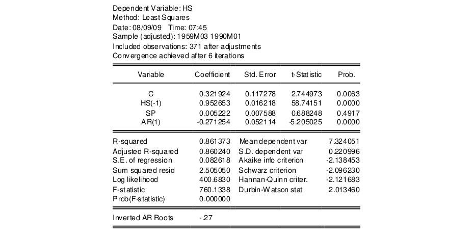
We estimate a regression of HS on a constant, SP, and the lag of HS, with an AR(1) to correct for residual serial correlation, using data for the period 1959M01–1990M01, and then use the model to forecast housing starts under a variety of settings. Following estimation, the equation results are held in the equation object EQ01:
Note that the estimation sample is adjusted by two observations to account for the first difference of the lagged endogenous variable used in deriving AR(1) estimates for this model.
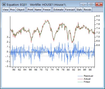
To get a feel for the fit of the model, select then choose Graph:
The actual and fitted values depicted on the upper portion of the graph are virtually indistinguishable. This view provides little control over the process of producing fitted values, and does not allow you to save your fitted values. These limitations are overcome by using EViews built-in forecasting procedures to compute fitted values for the dependent variable.
How to Perform a Forecast
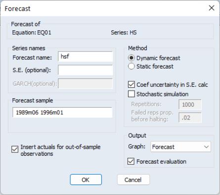
To forecast HS from this equation, push the button on the equation toolbar, or select .
At the top of the dialog, EViews displays information about the forecast. Here, we show a basic version of the dialog showing that we are forecasting values for the dependent series HS using the estimated EQ01. More complex settings are described in
“Forecasting from Equations with Expressions”.
You should provide the following information:
• . Fill in the edit box with the series name to be given to your forecast. EViews suggests a name, but you can change it to any valid series name. The name should be different from the name of the dependent variable, since the forecast procedure will overwrite data in the specified series.
• S.E. (optional). If desired, you may provide a name for the series to be filled with the forecast standard errors. If you do not provide a name, no forecast errors will be saved.
• GARCH (optional). For models estimated by ARCH, you will be given a further option of saving forecasts of the conditional variances (GARCH terms). See
“ARCH and GARCH Estimation” for a discussion of GARCH estimation.
• Forecasting method. You have a choice between and forecast methods.
Dynamic calculates
dynamic, multi-step forecasts starting from the first period in the forecast sample. In dynamic forecasting, previously forecasted values for the lagged dependent variables are used in forming forecasts of the current value (see
“Forecasts with Lagged Dependent Variables” and
“Forecasting with ARMA Errors”). This choice will only be available when the estimated equation contains dynamic components,
e.g., lagged dependent variables or ARMA terms.
Static calculates a sequence of
one-step ahead forecasts, using the actual, rather than forecasted values for lagged dependent variables, if available.
You may elect to always ignore coefficient uncertainty in computing forecast standard errors (when relevant) by unselecting the box.
In addition, in specifications that contain ARMA terms, you can set the Structural option, instructing EViews to ignore any ARMA terms in the equation when forecasting. By default, when your equation has ARMA terms, both dynamic and static solution methods form forecasts of the residuals. If you select , all forecasts will ignore the forecasted residuals and will form predictions using only the structural part of the ARMA specification.
• Sample range. You must specify the sample to be used for the forecast. By default, EViews sets this sample to be the workfile sample. By specifying a sample outside the sample used in estimating your equation (the estimation sample), you can instruct EViews to produce out-of-sample forecasts.
Note that you are responsible for supplying the values for the independent variables in the out-of-sample forecasting period. For static forecasts, you must also supply the values for any lagged dependent variables.
• Output. You can choose to see the forecast output as a graph (with either just the forecast values, or forecast values alongside actuals) or a numerical forecast evaluation, or both. Forecast evaluation is only available if the forecast sample includes observations for which the dependent variable is observed.
• Insert actuals for out-of-sample observations. By default, EViews will fill the forecast series with the values of the actual dependent variable for observations not in the forecast sample. This feature is convenient if you wish to show the divergence of the forecast from the actual values; for observations prior to the beginning of the forecast sample, the two series will contain the same values, then they will diverge as the forecast differs from the actuals. In some contexts, however, you may wish to have forecasted values only for the observations in the forecast sample. If you uncheck this option, EViews will fill the out-of-sample observations with missing values.
Note that when performing forecasts from equations specified using expressions or auto-updating series, you may encounter a version of the dialog that differs from the basic dialog depicted above. See
“Forecasting from Equations with Expressions” for details.