Wavelet Analysis
Many economic time series feature time-varying characteristics such as non-stationarity, volatility, seasonality, and structural discontinuities. Wavelet analysis is a natural framework for analyzing these phenomena without imposing simplifying assumptions such as stationarity. In particular, wavelet filters can decompose and reconstruct a time series, as well as its correlation structure, across time scales.
While wavelets have applications in diverse areas such as such as regression, unit root testing, bootstrapping (wavestrapping), and fractional integration order estimation, EViews focuses on four popular areas of application:
• Wavelet transforms
• Variance decomposition
• Outlier detection
• Thresholding (denoising)
Additional discussion of wavelet analysis is provided in
“Technical Background”.
Performing Wavelet Analysis in EViews
To perform wavelet analysis in EViews, open the series of interest and click on . There are four sub-menu entries corresponding to the four areas of application. We consider each in turn.
Wavelet Transforms
Typically, the first step in wavelet analysis is to perform a wavelet transform of some input series (discrete wavelet transform analysis is described in
“Discrete Wavelet Transform”).
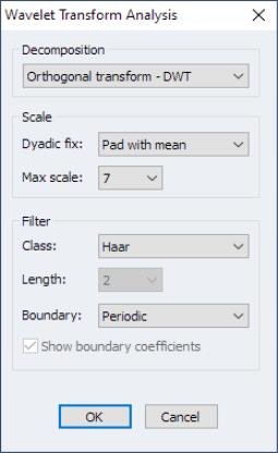
Click on to display the wavelet transform analysis dialog:
The first step is to choose a discrete wavelet decomposition type.
• The dropdown offers you a choice between the four supported methods:
1. (orthogonal discrete wavelet transform)
2. (non-orthogonal maximum overlap discrete wavelet transform)
3. (multiresolution analysis using a DWT transform)
4. (multiresolution analysis using a MODWT transform)
Next you may specify scale options:
• If you select a method that employs DWT and the input series is not of dyadic (power of 2) length, the dropdown will offer several options for adjusting the sample to derive the transform (
“Adjusting Non-dyadic Length Time Series”). You may choose between , , , and .
The padding methods add the specified value to the end of the input series to achieve the next dyadic length. The method truncates the input series at the preceding dyadic length.
• The dropdown lets you choose the maximum wavelet scale up to which the transform will be computed. The default is the maximum possible based on sample size. While the DWT is limited by sample size, the MODWT is not. Accordingly, if the transform method is one of MODWT or MODWT MRA, the maximum wavelet scale is specied as an input value.
Lastly, you may use the group settings to specify properties of the filter
• The dropdown specifies the choice of wavelet filter. You may select between , , and filters.
If you select either of the latter two filters, you will be prompted to provide a . The Daubechies class offers filter lengths running from 4 to 20 in increments of 2, whereas the symmlets offers filter lengths running from 8 to 20 in increments of 2
• The dropdown allows you to choose the method for handling boundary conditions resulting from circular recycling of observations. You may choose and .
The setting has the filter wrap around the end of the input series to handle endpoint missing observations. The setting concatenates the reverse of the input series to form an input of length

.
• By default, EViews will highlight boundary coefficients in the output. If you do not wish to highlight these values, uncheck the checkbox.
Example (Discrete Wavelet Transform)
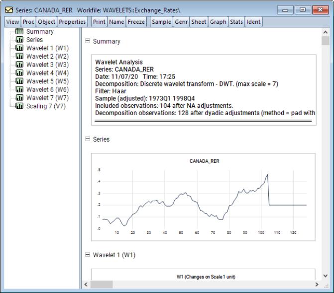
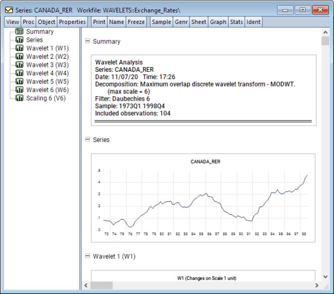
As a first example, consider the Canadian real exchange rate data extracted from the data set in Pesaran (2007) in “wavelets.WF1”. This is a quarterly series running from 1973q1 to 1998q4. We will use the default settings in the dialog. To display the transform, open the CANADA_RER series and select from the series window, click on .
Note that since the number of data points is 104, a dyadic adjustment is needed and the default setting pads the input series using the series mean is used to achieve dyadic length.
The output is a spool object with the spool tree listing the summary, original series, as well as wavelet and scaling coefficients for scales 1 through 7. The first of these is a summary of the wavelet transformation performed.
The second spool entry is a plot of the original series along with the padded values.
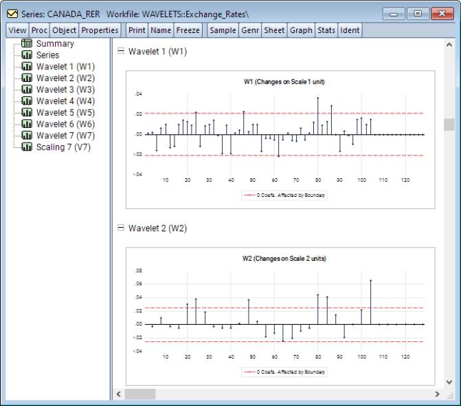
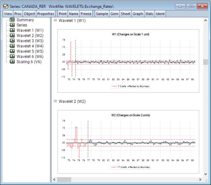
The remaining entries in the spool are wavelet and scaling coefficients plotted for each scale. Scroll down or click on an entry to bring it into view:
Here, we see the wavelet coefficients at scales 1 and 2. Notice that standard deviation of the coefficients at each plot has two dashed red lines. These represent the +/– standard deviation of coefficients at that scale. This is particularly useful in visualizing which wavelet coefficients should be shrunk to zero in wavelet shrinkage applications. Recall that coefficients exceeding some threshold bound (in this case the standard deviation) ought to be retained, whereas the remaining coefficients ought to be shrunk to zero.
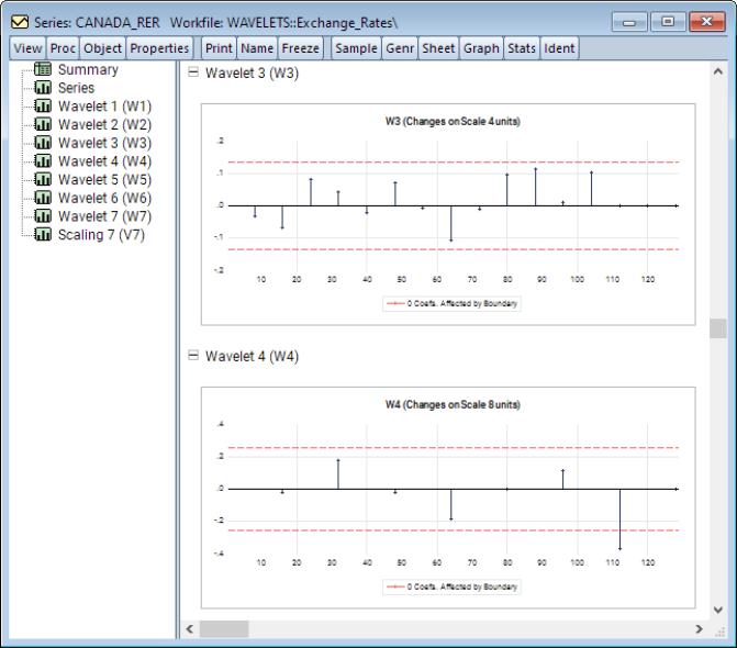
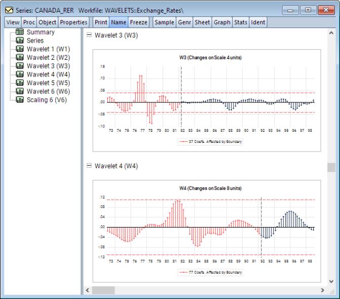
Continuing to higher scales, we see much smaller relative values
Looking at the wavelet coefficients at each scale, it is clear that the majority of relevant information can be captured only in the first few scales and using very few coefficients. For instance, at scale 1 we see roughly 3 or 4 wavelet coefficients which exceed the threshold bounds. Those are the coefficients which will contribute most to explaining variation at that scale and will capture the most transitory (noise) features of the underlying series. At scale 2, there are 6 coefficients which exceed the threshold bounds. While these coefficients are in the lower half of the frequency range, they are not in the immediate vicinity of frequency 0. We can conclude that this is a series which has persistence, but is not necessarily non-stationary. A quick unit root test will also confirm this belief.
Finally, notice that the time-axis in the DWT is not actually aligned with time, but rather the number of observations. This offset occurs because the filters used are in fact not zero-phase filters and therefore their transformation will not be aligned with time.
Example (Maximal Overlap Discrete Wavelet Transform)
For the second example, use the input series from the first example and perform a MODWT with the Daubechies filter of length 6. From the series window, click on . to display the dialog.
Then in the dropdown select . In the dropdown select and in the dropdown select 6. Click on .
As before, the output is a spool object with wavelet and scaling coefficients as individual spool elements.
• The first spool output is a summary of the transformation procedure.
• The second displays the series transform.
• The remainder of the output are the wavelet and scaling coefficients.
Note that since the MODWT is not an orthonormal transform and since it uses all of the available observations, wavelet and scaling coefficients are of input series length and do not require length adjustments.
Scrolling down or clicking on in the tree to bring the graph into view displays:
Next, notice that for each scale those coefficients affected by the boundary are displayed in red, and their count reported in the legends. Moreover, there is a dashed vertical line indicating the end of the boundary coefficients. Furthermore, since the MODWT is a redundant transform, the number of boundary coefficients standard deviation bounds will always be greater than those in the orthonormal DWT. As before the are available for reference. Finally, note that the time-axis in the MODWT is aligned with time. This is an advantage of the MODWT over the DWT at the expense of redundancy.
As in the DWT example, it's clear that the majority of relevant wavelet coefficients (those exceeding threshold bounds) are concentrated in the first few scales. We also observe that there are significantly more such coefficients in the MODWT transformation as opposed to the DWT since the MODWT is a redundant transformation and wavelet coefficients across scales are correlated. This behavior is also seen in the wave-like patterns in the output
Wavelet Variance Decomposition
Wavelet variance decomposition is described in
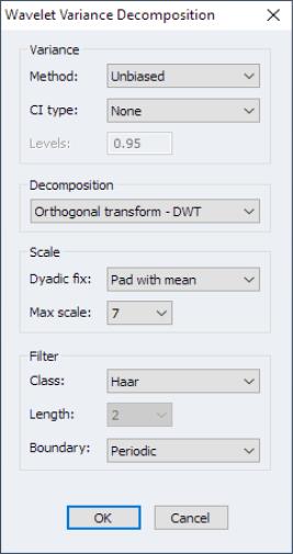
“Wavelet Analysis of Variance”. To perform wavelet decomposition of variance in EViews, open a series window and proceed to to display the dialog.
The group settings control the computation of the variances and confidence intervals:
1. – per-scale variance contributions using the unbiased variance form.
2. – per-scale variance contributions using the biased variance form.
When the variance decomposition is unbiased the maximum filter scale is adjusted automatically to reflect dropping boundary coefficients.
If the decomposition is unbiased, one can also form confidence intervals for per-scale variance contributions.
• The dropdown offers four choices:
1. – no confidence intervals are produced.
2. – confidence intervals are produced using Gaussian critical values
3. – confidence intervals are produced using Chi-squared critical values using equation and EDOF based on asymptotic estimation.
4. – confidence intervals are produced using Chi-squared critical values using equation and EDOF based on band-pass estimation.
• If a confidence interval will be computed, the field specifies the confidence interval coverage probability.
Lastly, the and group elements were discussed in detail in
“Wavelet Transforms”.
Example (Maximal Overlap Unbiased Variance Decomposition)
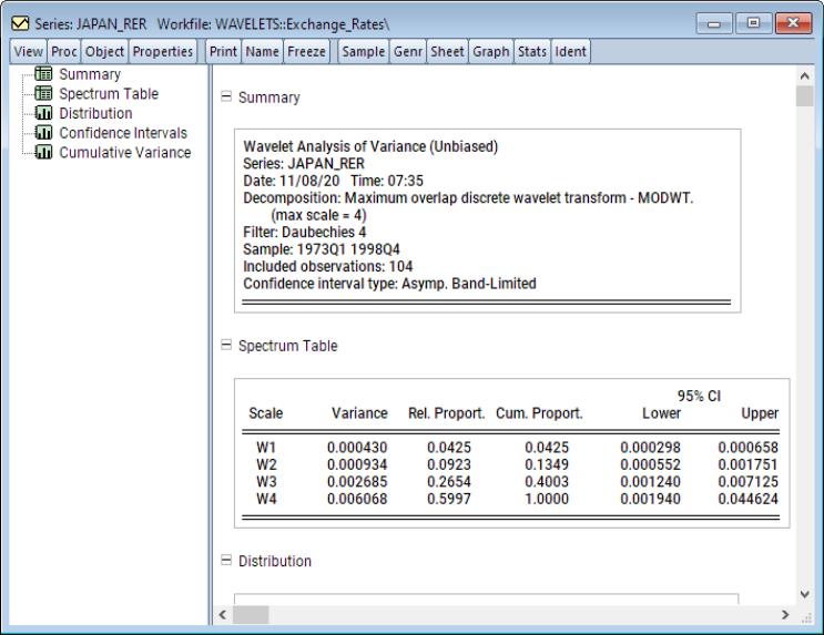
For this example, we use Japanese real exchange rate data from 1973Q1 to 1988Q4 extracted from the data set in Pesaran (2007). The objective is to produce a scale-by-scale decomposition of variance contributions using the MODWT with a Daubechies filter of length 4. Furthermore, we’ll produce a 95%confidence intervals using the asymptotic Chi-squared distribution using a band-pass estimate for the EDOF. The band-pass EDOF is preferred here since the sample size is less than 128 and the asymptotic approximation to the EDOF requires a sample size of at least 128 for decent results.
To proceed, open the series window and click on First, set the dropdown to . Next, set the dropdown in the group to Lastly, change the group dropdown to and click on to display the results.
The output is a spool object with the spool tree listing the procedure summary, energy spectrum, variance distribution across-scales, CIs across scales, and the cumulative variance.
The first spool entry is a summary of the wavelet variance decomposition performed including information about the decomposition and filter, sample, and the confidence intervals settings.
The second entry is a table of the variance spectrum listing the contribution to overall variance by wavelet coefficients at each scale. The column titled “Variance” shows the variance contributed to the total at a given scale. Columns titled “Relative Proportion” and “Cumulative Proportion” display the proportion of overall variance contributing to the total at a given scale and its cumulative total, respectively.
Here, since confidence intervals have been produced, the last two columns display the lower and upper confidence interval values at each scale.
We may scroll down or click on the selector to view the next items in the spool:
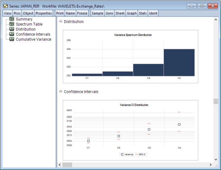
The next object in the spool is the graph, which is a bar plot of variances at each given scale.
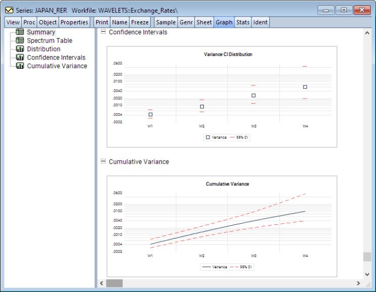
Following this is the graph, which shows the variance values along with their 95% confidence intervals at each scale.
Scrolling down to the last graph or clicking on , we see a display showing the cumulative variances across scales and, if computed, the cumulative confidence interval.
Wavelet Threshold (Denoising)
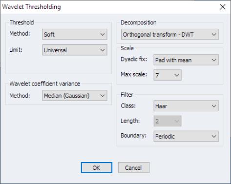
As in the previous wavelet examples, wavelet thresholding in EViews is performed on a series. In particular, from an open series window, click on to display the dialog.
The group options control the specification of the threshold:
• The dropdown controls the method for determining the optimal threshold value. You may select between , , , , and (
“Threshold Value Methods” )
The group specifies the method for computing the estimate of the variance (standard deviation) of the wavelet coefficients
The remaining and group elements were discussed in detail in
“Wavelet Transforms”.
Example (Discrete Wavelet Hard Thresholding)
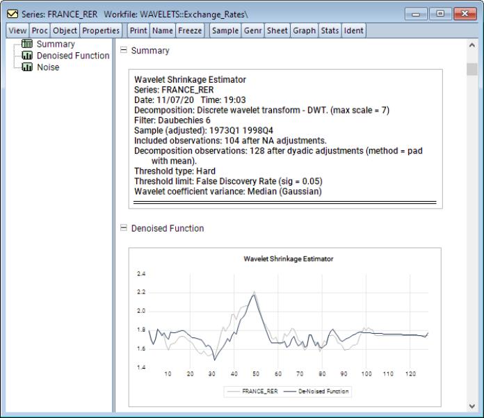
For our example, we use the French real exchange rate data from 1973q1 to 1988q4 extracted from the data set in Pesaran (2007). The objective is to de-noise the input function by extracting its signal using the DWT with a Daubechies filter of length 6. We will employ a hard thresholding rule using a false discovery rate threshold with significance level 05. The wavelet variances will be estimated using the median with a Guassian correction.
To proceed, open the series window and click on
Under the group, set the dropdown to and set the dropdown to . Next, Under the group set the dropdown to . Lastly, change the dropdown to and set the dropdown to 6. Click on .
EViews displays spool output with a tree listing the summary, denoised function, and noise.
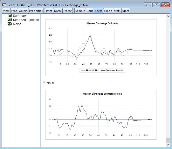
Finally, the remaining plot is the noise process extracted from the original series.
At the top of the spool is a summary of the denoising procedure describing the decomposition method and filter, sample information, threshold method, and wavelet coefficient variance computation.
Below the summary information is a plot of the denoised function (signal) superimposed over the original series.
Scrolling down or clicking on the entry on the left-hand side of the spool brings the graph of the noise (difference) into view.
Wavelet Outlier Detection
Wavelet outlier detection is described in
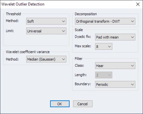
“Wavelet Outlier Detection”. To perform wavelet outlier detection in EViews, open a series window and proceed to to display the dialog.
The dialog is identical to the dialog described in
Example (Discrete Wavelet Transform Outlier Detection)
To demonstrate outlier detection, we employ data obtained from the U.S. Geological Survey website https://www.usgs.gov/.
As discussed in Bilen and Huzurbazar (2002), data collected in this database comes from many different sources and is generally notorious for input errors. Here we focus on a monthly dataset, collected at irregular intervals from Mary 19876 to June 2020, measuring water conductance at the Green River near Greendale, UT, identified by site number 09234500.
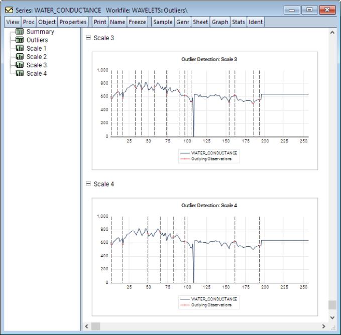
A quick glance at the series indicates that there is an unusually large drop from typical values (500 to 800 units) in September 1999 which drops to roughly 7.4 units. This is an unusually large drop and is almost certainly an outlying observation. In an attempt to identify the aforementioned outlier and perhaps uncover others, the example conducts the Bilen and Huzurbazar (2002) wavelet outlier detection using a DWT transform with a Haar filter, universal threshold, and a mean median absolute deviation estimator for wavelet coefficient variance. Furthermore, the maximum decomposition level is restricted to 3.
To proceed, open the series window and click on View/Wavelet Analysis/Outlier Detection.... Change the Max Scale to 4 and under the MAD group, set the Method to Mean Median Abs. Dev., and click on OK.
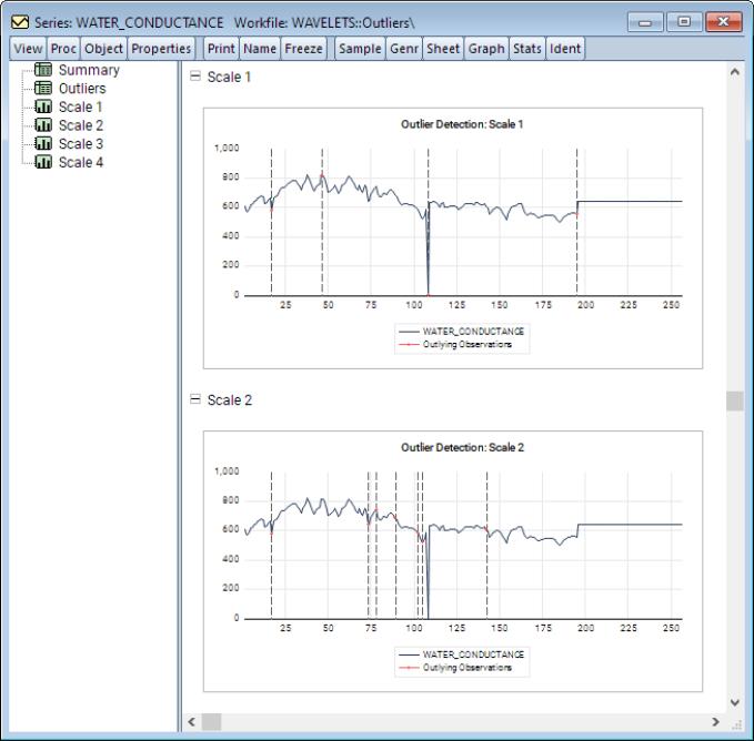
EViews will display output in the form of a spool object with the spool tree listing the summary, outlier table, and outlier graphs for each of the relevant scales.
The first spool entry is a summary of the outlier detection procedure describing the decomposition method and filter, sample information, threshold method, and wavelet coefficient variance computation.
Next is an outlier overview table listing the exact location of a detected outlier along with its value and absolute deviation from the series mean and median, respectively.
We may scroll down or click on one of the scale entries on the left-hand side to display graphs of the outliers.
These graphs show, for each scale, plots of the original series with red dots and dotted vertical lines identifying outlying observations.
Saving Results to the Workfile
If you wish to save the wavelet results to the workfile you may click on
For discussion, see
“Wavelet Objects”.
Technical Background
Many economic time series feature time-varying characteristics such as non-stationarity, volatility, seasonality, and structural discontinuities. Wavelet analysis is a natural framework for analyzing these phenomena without imposing simplifying assumptions such as stationarity. In particular, wavelet filters can decompose and reconstruct a time series, as well as its correlation structure, across time scales. Moreover, these decompositions can be orthogonalized so that a decomposition at one scale is uncorrelated with a decomposition at another. This property is clearly useful in isolating features associated with a given timescale, as well as achieving de facto decomposition and preservation of variation akin to eigenvalue diagonalization in principal component analysis.
Wavelet analysis is analogous, in many ways, to Fourier spectral analysis as both methods can represent a time series signal in a different space. This is achieved by expressing, to a desired degree of precision, the time series signal as a linear combination of basis functions.
For Fourier analysis, these basis functions are sines and cosines. These functions approximate global variation well, but are poorly adapted to modeling local time-variation, and to capturing discontinuous, non-linear, and non-stationary processes whose impulses persist and evolve with time.
Accordingly, Fourier basis functions approximate global variation well. Nevertheless, local variation, otherwise known as time-variation in time-series, is poorly adapted to cylical functions such as the sinus and cosinus. Accordingly, the trigonometric basis functions are ideally adapted to stationary processes characterized by impulses which wane with time, but are poorly adapted to discontinuous, non-linear, and non-stationary processes whose impulses persist and evolve with time. The Fourier transform is localized well in frequency, but lacks good time resolution. Furthermore, if components captured at a given frequency are non-stationary and time-dependent, then attempting to capture all such components with a single frequency (which is itself time independent), will clearly not work very well. To surmount this time-frequency relationship, a new set of basis functions are needed.Alternatively, the wavelet transform, and therefore the wavelet basis functions, are localized both in scale and time. In particular, the latter form a set of shifts and dilations of a
mother wavelet function 
which is any function satisfying:
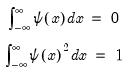 | (42.125) |
We say that wavelets have mean zero and unit energy. The term energy originates in the signal processing literature, and is formalized as
 | (42.126) |
for some function

. The term is interchangeable with the familiar
variance for non-complex functions. Wavelet basis functions assume the form:
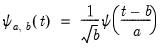 | (42.127) |
where

is the location constant, and

is the scaling factor (which corresponds to the notion of frequency in Fourier analysis). Wavelet transforms are well-adapted to non-stationary and discontinuous phenomena since both scale and time resolutions are preserved.
Since wavelet basis functions are de facto location and scale transformations of a single function, they are an ideal tool for multiresolution analysis (MRA)–the ability to analyze a signal at different frequencies with varying resolutions.
Moving along the time domain, MRA allows one to zoom to a desired level of detail such that high (low) frequencies yield good (poor) time resolutions and poor (good) frequency resolutions. Since economic time series often exhibit multiscale features, wavelet techniques can decompose these series into constituent processes associated with different time scales.
Discrete Wavelet Transform
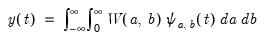
In the context of continuous functions, the continuous wavelet transform (CWT) of a time series

is defined as
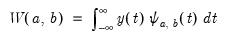 | (42.128) |
and the inverse transformation for reconstructing the original process is
 | (42.129) |
See Percival and Walden (2000) for a detailed discussion.
Since continuous functions are rarely observed, a discretized analogue of the CWT is generally employed. The discrete wavelet transform (DWT) is a collection of CWT “slices” at nodes
such that

,

, where

, for dyadic observation length

for

. The resulting discrete wavelet basis function is of the form
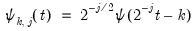 | (42.130) |
Unlike the CWT which is highly redundant in both location and scale, the DWT can be designed as an orthonormal transformation. If the location discretization is restricted to the index
, at each scale

, half the available observations are lost in exchange for orthonormality. This is the classical DWT framework. Alternatively, if the location index is restricted to the full set of available observations with

, the discretized transform is no longer orthonormal, but does not suffer from observation loss. The latter framework is typically referred to as the
maximal overlap discrete wavelet transform (MODWT), and sometimes as the
non-decimated DWT.
Mallat’s Pyramid Algorithm
In practice, the DWT proceeds as a filtering operation (both low and high pass) on a time series, following the pyramid algorithm of Mallat (1989).
In case of the classical DWT with

, let
and define the matrix of DWT coefficients
. Here,

is a vector of wavelet coefficients of length

and is associated with changes on a scale of length

. Moreover,

is a vector of scaling coefficients of length

and is associated with averages on a scale of length ‑

. Furthermore,

where
is some

orthonormal matrix generating the DWT coefficients.
The algorithm convolves an input signal with wavelet high and low pass filter coefficients to derive the
j-th level DWT matrix
. In particular, each iteration

convolves the scaling coefficients from the preceding iteration, namely

, with both the high and low pass filter coefficients. The input signal in the first iteration is

. The entire algorithm continues until the

-th iteration, although it can be stopped earlier.
Wavelet Filters
Like traditional filters which are used to extract components of a time series such as trends, seasonalities, business cycles, and noise, wavelets filters perform a similar role. Like traditional filters, wavelet filters are also designed to capture low and high frequencies, and have a particular length. This length governs how much of the original series information is used to extract low and high frequency phenomena. The role of the length is very similar to the role of the autoregressive (AR) order in traditional time series models where higher AR orders imply more historical observations influence the present.
The simplest and shortest wavelet filter is of length

and is called the Haar wavelet. This is a sequence of rescaled rectangular functions and is therefore ideally suited to analyzing signals with sudden and discontinuous changes. In this regard, it is ideally suited for outlier detection. Unfortunately, the Haar filter is typically too simple for most other applications.
In contrast, Daubechies (1992) introduced a family of filters of even length that are indexed by the polynomial degree they are able to capture – rather the number of vanishing moments. Thus, the Haar filter, which is of length 2, can only capture constants and linear functions. The Daubechies wavelet filter of length 4 can capture everything from a constant to a cubic function. Accordingly, higher filter lengths are associated with higher smoothness.
It should be noted that Daubechies (1992) filters, also known as daublets, are typically not symmetric. If a more symmetric version of the daublet filters is required, then the class known as least asymmetric, or symmlets, is used.
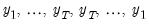
Boundary Conditions
It’s important to note that both the DWT and the MODWT make use of circular filtering. In particular, when a filtering operation reaches the beginning or end of an input series, otherwise known as the boundaries, the filter treats the input time series as periodic with period

. In other words, we assume that
, are useful surrogates for unobserved values

. Those wavelet coefficients which are affected by this circularity are also known as
boundary coefficients. Note that the number of boundary coefficients only depends on the filter length

and is independent of the input series length

. Furthermore, the number of boundary coefficients increases with filter length

. Both DWT and MODWT boundary coefficients will appear the beginning of

and

. You may refer to Percival and Walden (2000) for further details.
Multiresolution Analysis
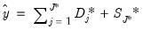
Similar to Fourier, spline, and linear approximations, a principal feature of the DWT is the ability approximate an input series as a function of wavelet basis functions. The general idea in wavelet theory is termed
multiresolution analysis (MRA) and refers to the approximation of an input series at each scale (and up to all scales)

. For each
,
 | (42.131) |
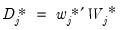
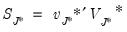
where the

and
are

-dimensional vectors of the
j-th level
detail and the

-th level
smooth series. Furthermore, since the low-pass (high-pass) wavelet coefficients are associated with changes (averages) at scale

, the detail and smooth series are associated with changes and average at scale

, respectively, in the input series

.
The MRA is typically used to derive approximations for the original series using its lower and upper frequency components. Since upper frequency components are associated with transient features and are captured by the wavelet coefficients, the detail series will in fact extract those features of the original series which are typically associated with “noise”. Alternatively, since lower frequency components are associated with perpetual features and are captured by the scaling coefficients, the smooth series will in fact extract those features of the original series which are typically associated with the “signal”.
It’s worth mentioning here that since wavelet filtering can result in boundary coefficients, the detail and smooth series will also have observations affected by the boundary.
Wavelet Analysis of Variance
The orthonormality of the DWT generating matrix

has important implications. In particular, the DWT is an energy (variance) preserving transformation. Coupled with this preservation of energy is the decomposition of energy on a scale-by-scale basis. Then,
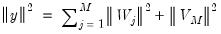 | (42.132) |
where

is the Euclidean norm. Thus,

quantifies the energy of

accounted for at scale

.
This energy decomposition is known as the wavelet power spectrum (WPS) and is arguably the most important of the properties of the DWT, and bears resemblance to the spectral density function (SDF) used in Fourier analysis.
The total variance in

can be decomposed as
 | (42.133) |
where

is the contribution to

due to scale

, and is estimated as
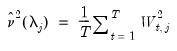 | (42.134) |
since

is the contribution to the sample variance of

at scale

.
Unfortunately, this estimator is biased due to the presence of boundary coefficients. To derive an unbiased estimate, boundary coefficients should be dropped from consideration. Accordingly, an unbiased estimate of the variance contributed at scale

is given by
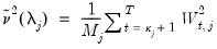 | (42.135) |
where

and

represents the number of coefficients affected by boundary conditions.
Variance Confidence Intervals
It is also possible to derive confidence intervals for the contribution to the overall variance at each scale.
An asymptotic normal confidence interval is given by
 | (42.136) |
where
 | (42.137) |
and

is the integral of the squared spectral density function of wavelet coefficients

excluding any boundary conditions. As shown in Percival and Walden (2000),

can be estimated as the sum of squared serial correlations among

excluding boundary coefficients. Priestly (1981) notes that there is no condition that prevents the lower bound of this confidence interval from becoming negative.
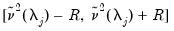
Percival and Waldon (2000) employ an asymptotic Chi-square confidence interval
 | (42.138) |
where

is the

-quantile of the

distribution and

is the equivalent degrees of freedom (EDOF) which may be estimated using one of two suggestions
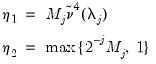 | (42.139) |
The first estimator,

, relies on large sample theory, and in practice requires a sample of at least

to yield a decent approximation. The second estimator,

, assumes that the spectral density function of the wavelet coefficients at scale

is a
band-limited. See Percival and Walden (2000) for detail.
Wavelet Outlier Detection
A particularly important and useful application of wavelets is outlier detection. While the subject matter has received some attention over the years starting with Greenblatt (1996), here we focus on a rather simple and appealing contribution by Bilen and Huzurbazar (2002).
The appeal of the Bilen and Huzurbazar approach is that it doesn’t require model estimation, is not restricted to processes generated via ARIMA, and works in the presence of both additive and innovational outliers. The approach also assumes that wavelet coefficients are approximately independent and identically normal variates. While EViews offers the ability to perform this procedure using a MODWT, it’s generally better suited to the DWT. Moreover, Bilen and Huzurbazar suggest that Haar is the preferred filter since the latter yields coefficients large in magnitude in the presence of jumps or outliers. They also suggest that the transformation be carried out only at the first scale.
The overall procedure works on the principle of thresholding and the authors suggest the use of the universal threshold. The idea here is that extreme (outlying) values will register as noticeable spikes in the spectrum. These spike generating values are outlier candidates.
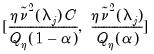
For

, the number of wavelet coefficients at scale

, the outlier detection algorithm is given by:
1. Compute a wavelet transformation of the original data up to some scale

.
2. Select an optimal threshold

.
3. For

find the set of indices
such that

for
4. Find the exact location of the outlier among the original observations. For instance, if

is an index associated with an outlier:
• If the wavelet transform is the DWT, the original observation associated with that outlier is either

or

. To choose between the two, let

denote the mean of the original observations excluding those two values. Between the two candidates, the outlier is the one which has the largest absolute deviation from

.
• If the wavelet transform is MODWT, the outlier is the observation indexed by

.
See Bilen and Huzurbazar (2002) for additional detail and discussion.
Wavelet Shrinkage (Thresholding)
A key objective in any empirical work is to discriminate noise from useful information. Suppose that the observed time series

where

is an unknown signal of interest obscured by the presence of unwanted noise

. Traditionally, signal discernment was typically achieved using discrete Fourier transforms. Naturally, this assumes that any signal is an infinite superposition of sinusoidal functions; a strong assumption in empirical econometrics where most data exhibits unit roots, jumps, kinks, and various other non-linearities.
The principle behind wavelet-based signal extraction, otherwise known as wavelet shrinkage, is to shrink any wavelet coefficients not exceeding some threshold to zero and then exploit the MRA to synthesize the signal of interest using the modified wavelet coefficients. In other words, only those wavelet coefficients associated with very pronounced spectra are retained with the additional benefit of deriving a very sparse wavelet matrix.
Thresholding Rule
The two most popular thresholding rules are
• Hard Thresholding (“kill/keep” strategy)
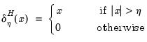 | (42.140) |
• Soft Thresholding
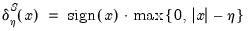 | (42.141) |
Threshold Value Methods
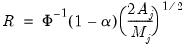
The threshold value

is the key to wavelet shrinkage. In particular, optimal thresholding is achieved when

, the standard deviation of the noise process

. There are several strategies for determining the optimal threshold:
• (Donoho and Johnstone 1994),
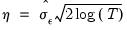 | (42.142) |
where

is estimated using wavelet coefficients only at scale

, regardless of the scale under consideration. When this threshold rule is coupled with soft thresholding, the combination is commonly referred to as
VisuShrink.
• (Donoho and Johnstone 1994),
 | (42.143) |
where

is the familiar average mean squared error measurement of risk. Unfortunately, a closed form solution for this approach is not available, although tabulated values exist. When this threshold rule is coupled with soft thresholding, the combination is commonly referred to as
RiskShrink.
• - SURE (Donoho and Johnstone 1994; Jansen 2010),
 | (42.144) |
where
and

is the mean of some variable of interest,

for

. In the framework of wavelet coefficients,

represents the wavelet coefficients at a given scale.
Furthermore, while the optimal threshold

based on this rule depends on the thresholding rule used, the solution may not be unique, so the SURE threshold value is the minimum of the

. In case of the soft thresholding rule, the solution was proposed in Donoho and Johnstone (1994). For the hard thresholding rule, the solution was proposed in Jansen (2010).
• (Abramovich and Benjamini 1995), determines the optimal threshold value through a multiple hypothesis testing problem. For further detail, see Donoho and Johnstone (1995), Donoho, Johnstone et al. (1998), Gençay, Selçuk andWhitcher (2001), and Percival and Walden (2000).
Wavelet Coefficients Variance
There remains the issue of how to estimate the variance of the wavelet coefficients

. If the assumption is that the observed data

is obscured by some noise process

, the usual estimator of variance will exhibit extreme sensitivity to noisy observations.
Let

and

denote the mean and median, respectively, of the wavelet coefficients

at scale

, and let

denote its cardinality (total number of coefficients at that scale). Then, several common estimators have been proposed in the literature:
• Mean Absolute Deviation
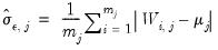 | (42.145) |
• Median Absolute Deviation
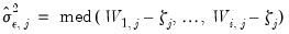 | (42.146) |
• Mean Median Absolute Deviation
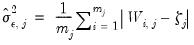 | (42.147) |
• Median (Gaussian)
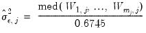 | (42.148) |
Thresholding Implementation
Given choice of the thresholding rules and optimal threshold value, all wavelet thresholding procedures involve the following:
1. Compute a wavelet transformation of the original data up to some scale

so that you obtain the wavelet and scaling coefficients
.
2. Select an optimal threshold

.
3. Threshold the coefficients at each scale

for
using the selected threshold value and rule. This procedure will generate a set of modified wavelet and scaling coefficients
.
4. Use MRA with the thresholded coefficients to generate an estimate of the signal:
 | (42.149) |
where the
and
Practical Considerations
The discussion above outlines the basic theory underlying wavelet analysis. Nevertheless, there are several practical (empirical) considerations which should be addressed. We focus here on three in particular: 1) selecting a wavelet filter, 2) handling non-dyadic series lengths, and 3) awareness of boundary conditions.
Choice of Wavelet Filter
The type of wavelet filter is typically chosen to mimic the data to which it is applied. Shorter filters don’t approximate the ideal band pass filter well, but longer ones do. On the other hand, if the data are derived from piecewise constant functions, the Haar wavelet or other shorter wavelets may be more appropriate. Alternatively, if the underlying data is smooth, longer filters may be more appropriate. In this regard, it’s important to note that longer filters expose more coefficients to boundary condition effects than
shorter ones. Accordingly, the rule of thumb strategy is to use the filter with the smallest length that gives reasonable results. Furthermore, since the MODWT is not orthogonal and its wavelet coefficients are correlated, wavelet filter choice is not as vital as for orthogonal DWT. Nevertheless, if alignment to time is important (i.e. zero phase filters), the least asymmetric family of filters may be a good choice.
Handling Boundary Conditions
Recall that wavelet filters exhibit boundary conditions due to circular recycling of observations. Although this may be an appropriate assumption for series with naturally exhibiting cyclical effects, it is not appropriate in all circumstances. An alternative approach is to reflect the original series to generate a series of length

so that filtering proceeds using observations
.
Whatever the approach, wavelet analysis should quantify how many wavelet coefficients are affected by boundary conditions.
Adjusting Non-dyadic Length Time Series
Recall that the DWT requires an input series of dyadic length. Naturally, this condition is rarely satisfied in practice. Broadly speaking, there are two approaches: either shorten the input series to dyadic length at the expense of losing observations, or “pad” the input series with observations to achieve dyadic length.
Although the choice of padding values is ultimately arbitrary, there are three popular choices, none of which has proven superior: 1) pad with zeros, 2) pad with mean, 3) pad with median.