Estimating ARDL and NARDL in EViews
EViews provides an powerful interface for ARDL and NARDL estimation.
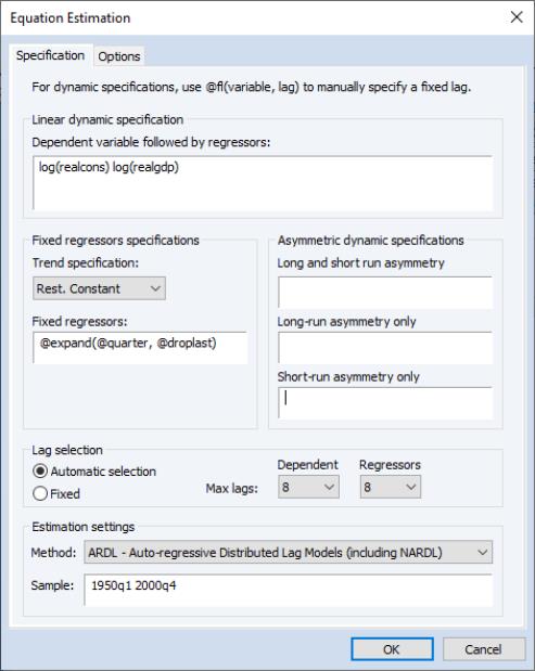
From the main EViews menu, click on or type the command equation in the command line to open the equation dialog. Then select the from the dropdown to display the tab of the ARDL dialog:
• In the first edit field under , you should a enter a list of variables consisting of the dependent variable followed by any symmetric ARDL distributed lag regressors. At a minimum, the edit field must contain the dependent variable.
• Exogenous regressors, including deterministics, may be specified in the section. Trend regressors corresponding to the five deterministic cases discussed in
“Bounds Test View” (, , , , ) may be specified using the dropdown. All other exogenous regressors (those apart from the constant and the trend) should be specified in the edit field.
• Asymmetric distributed lag regressors may be listed under . In particular, the edit field may be used to specify regressors which are asymmetric in both the long-run and short-run. Regressors which are asymmetric only in the long-run may be specified in the edit field, while those which are asymmetric exclusively in the short-run are specified in the edit field.
• The section specifies the lags for the dependent variable and the distributed lag regressors. By default, EViews uses automatic lag selection for both, following the PSS(1999), the lag structure of a ARDL model is chosen optimally using standard model selection criteria. You may use the dropdown menu on the page to select your criterion, choosing between using Akaike (AIC), Schwarz (BIC), Hannan-Quinn (HQ), or the adjusted

. Alternately, you may select the radio button for to provide user-specified lags. Given your choice of method, you may then use the dropdown menus to specify the actual or to be used for the variable or the distributed lag .
For automatic lag selection, if

and

are the maximum number of lags of the dependent and explanatory variables, and

is the total number of distributed-lag regressors, the total number of model evaluations is

; the number of combinations of the set of numbers

and

additional numbers from

. For example, with 2 distributed-lag regressors and

, the total number of considered models is 100.
When specifying the maximum number of lags, bear in mind that the ARDL model selection process will use the same sample for each estimation so that observations will be dropped from each candidate estimation based on the specified maximum. Once the lags are chosen, the final estimation output will use all observations available for the selected model. Thus, the final estimates will generally employ more observations than the model that was estimated during selection, and will be different than the selection model results.
• Additionally, you can override the global lag specification for individual variables. You may specify the lag for an individual variable using the “@fl(variable, lag)” syntax. For instance, if the variable X should use 3 lags, irrespective of the fixed or automatic lag settings, you may specify this by entering “@fl(x, 3)” in the regressor list.
• The tab of the estimation dialog allows you to specify the type of model selection to be used if you chose automatic lag selection. You may choose between the , , , or the objective.
• You may also select the type of covariance matrix to use in the final estimates, using the Coefficient covariance matrix dropdown. You may choose between , , and covariance estimation, and specify whether or not to perform a . Note that these settings do not affect the model selection criteria.
By default, linear ARDL estimation results are displayed using the IDT representation
Equation (29.1) while nonlinear ARDL estimates are displayed using the Conditional Error Correction (CEC) form
Equation (29.17). You may display the CEC and EC representations of a linear model using the
“Error Correction Output View” as described below.
For example, in these linear ARDL results, note that the dependent variable LOG(REALCONS) in the IDT representation is in levels,
Alternately for a nonlinear ARDL the CEC results are for a dependent variable in differences:
Note that the nonlinear results include entries for the special cumulative positive and negative difference transformations (@cumdp and @cumdn) of the nonlinear regressor LOG(REALGOVT). For brevity, the initialization date for the @cumdp and @cumdn cumulative difference functions is not displayed in the output. You may view this date using the full representation of the equation by clicking on from the estimated equation.