Background
If

is the dependent (autoregressive) variable,

are

distributed-lag explanatory variables, and

are

exogenous, potentially deterministic variables, the
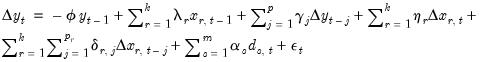
Intertemporal Dynamics (ITD) representation of an ARDL(

) model is given by:
 | (29.1) |
where

are the innovations, and

,

, and

are the coefficients associated with the exogenous variables,

lags of

, and

lags of the

distributed lag regressors

, respectively.
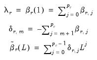
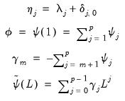
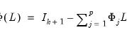
Let

be the usual lag operator and define the lag polynomials:
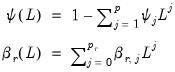 | (29.2) |
Substituting into
Equation (29.1) yields:
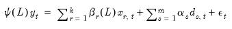 | (29.3) |
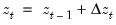
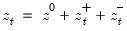
Noting that any series

may be written as
and performing a Beveridge-Nelson decomposition on both

and the

in
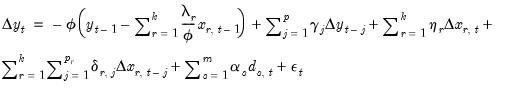
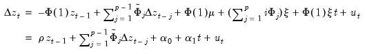
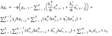
Equation (29.3) produces the
Conditional Error Correction (CEC) representation of the ARDL,
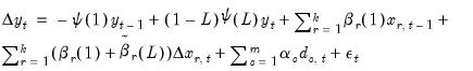 | (29.4) |
which, with a bit of manipulation, may be rewritten as
 | (29.5) |
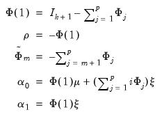
where
 | (29.6) |
and
 | (29.7) |
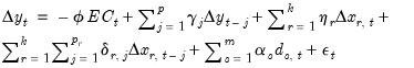
Since CEC
Equation (29.5) and
Equation (29.8) are derived from ITD
Equation (29.1), there is an obvious one-to-one correspondence between the two. As with the vector error correction (VEC) form of a VAR, the CEC form offers easy identification of a cointegrating relationship between the dependent variable and the explanatory variables in the ARDL. We discuss this parallel in greater depth in
“Relationship to Vector Error Correction (VEC) Models”.
Rearrange terms, we may re-write
Equation (29.8) as
 | (29.8) |
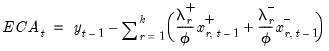
If we define the equilibrium error correction term,
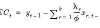 | (29.9) |
then
Equation (29.8) may be written in Error Correction (EC) form:
 | (29.10) |
where

is the error correction parameter, and the long-term equilibrium parameters for the explanatory variables are given by

, for

.
Conveniently, the coefficients in both the ITD and the CEC representations of the ARDL model may be estimated via least squares.
Relationship to Vector Error Correction (VEC) Models
Assuming the same lag across the distributed-lag regressors

and that the deterministics

consist of a simple constant and linear trend, Pesaran (2001) demonstrates that the ARDL CEC representation in
Equation (29.8) is in fact the CEC of the VAR(

) model:
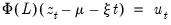 | (29.11) |
where
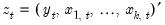
is a

vector of endogenous variables,

and

are the

vectors of intercept and trend coefficients, respectively, and
 | (29.12) |
is the

matrix lag polynomial.
Invoking the BN decomposition on

and with following some rearrangement, the CEC representation of this VEC may be written as
 | (29.13) |
where
 | (29.14) |
which is equivalent to
Equation (29.5).
Nonlinear (asymmetric) ARDL
The classical ARDL framework assumes that the long-run relationship

is a symmetric linear combination of regressors. While this is a natural starting assumption, it does not match the behavioral finance and economics literature approach to modeling nonlinearity and asymmetry (Kahneman, Tversky, and Shiller, 1979). In response, Shin (2014) proposes a nonlinear ARDL (NARDL) framework in which short-run and long-run nonlinearities are modeled as positive and negative partial sum decompositions of the explanatory variables.
Consider the partial sum decomposition of a variable

around a threshold of

as
where

and

are the partial sum processes of positive and negative
changes in

, respectively:
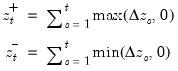 | (29.15) |
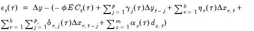
The ITD representation of a NARDL(

) model is given by:
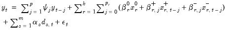 | (29.16) |
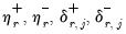
where

are coefficients for the initial conditions, and where

and

are coefficients associated with the asymmetric distributed-lag variables.
We may an obtain a CEC representation of the ITD NARDL model,
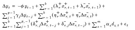 | (29.17) |
where the
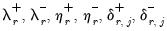
are asymmetric analogues of the coefficients in
Equation (29.6).
We may rearrange terms so that
Equation (29.17) becomes
 | (29.18) |
Then, define the asymmetric equilibrium error correction term,
 | (29.19) |
so that the CEC
Equation (29.18) may be written in EC form:
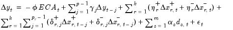 | (29.20) |
where

is the error correction parameter, the long-term equilibrium parameters for the explanatory variables are given by

and

for

. The short-run parameters for the explanatory variables are given by the
.
Notice that because the CEC representation decomposes the effect of the distribution lag variables into short and long-run components, it allows for asymmetries in various combinations of short and long-run dynamics. This flexibility does not exist in the ITD representation.
As with their symmetric counterparts, NARDL models may be estimated via least squares. This result is appealing since nonlinear models often require iterative estimation routines. Furthermore, bounds testing procedures (
“Bounds Test View”) remain valid and require no meaningful adjustments.
Quantile ARDL (QARDL)
The Quantile Autoregressive Distribued Lag (QARDL) model, introduced by Cho, Kim, and Shin (2015), is an modification of traditional ARDL models to capture the dynamics of conditional quantiles (percentiles) of the dependent variable. While conventional models provide insights into the mean responses of the dependent variable to changes in predictors, QARDL models model the effects of changes in predictors on the quantiles of the dependent variable.
This shift in focus onto quantiles may offer additional insight into the relationship between predictor and dependent variable. While a traditional ARDL model might suggest that an increase in

leads to an average increase in

, the QARDL may reveal that the increase is more pronounced at higher percentiles and subdued at lower ones. This granularity is invaluable in scenarios where the impact of shocks or policy changes might differ across various segments of a distribution.
Similarly, a study of economic policy on income levels will often suggest that certain policies disproportionately benefit higher income brackets (higher quantiles) more than lower brackets (lower quantiles), or vice versa. Likewise, financial markets assessing risk are often interested in extreme behavior which we may model using extreme quantiles (e.g., the 1st or 99th percentile).
We model the

-th conditional quantile of

as
 | (29.21) |
and define the quantile residual as
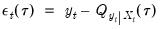 | (29.22) |
The Quantile Autoregressive Distributed Lag (QARDL) estimator is given by:
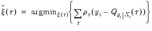 | (29.23) |
where
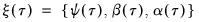
and
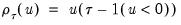
is the so-called
check function which weights positive and negative values asymmetrically.
This conditional quantile specification in
Equation (29.21) is obviously analogous to the traditional ARDL specification for the mean given in
Equation (29.1) and the QARDL model is essentially a traditional ARDL specification estimated using quantile regression (see
“Quantile Regression” for an overview of quantile regression estimation).
Since QARDL is simply a specific case of quantile regression, all of the tools of quantile regression estimation, such as quantile process visualization and quantile equality and symmetry tests, apply in the QARDL framework.
Further, since QARDL is an ARDL model applied to conditional quantiles, conventional ARDL results apply so that standard diagnostic tests, cointegration tests, and error correction mechanisms carry over to QARDL. Notably, since the coefficients defining the Intertemporal Dynamics (ITD) and Conditional Error Correction (CEC) representations of the traditional ARDL model are quantile specific, the QARDL error correction form is given by
 | (29.24) |
for error correction term
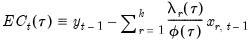 | (29.25) |
where all of the coefficients are quantile regression analogues for the corresponding coefficients defined in
Equation (29.6) and
Equation (29.7) in the ARDL error correction framework.
Note that quantile regression may also be extended to encompass the Nonlinear ARDL (NARDL) as in
“Nonlinear (asymmetric) ARDL”. The QNARDL analogue of the NARDL error-correction equation
Equation (29.20) is
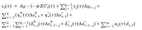 | (29.26) |
where the quantile error correction term is
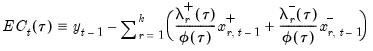 | (29.27) |
and the
are asymmetric analogues of the coefficients in
Equation (29.6).
The asymmetric long-run quantile process associated with the distributed-lag variables are

and

. The short-run parameters for the explanatory variables are given by
.