Views and Procs of ARDL
Since ARDL and NARDL models are estimated by simple least squares, all of the views and procedures available to equation objects estimated by least squares are also available for ARDL models. There there are a few ARDL specific issues, view, and procs that require additional discussion.
Model Selection Summary
The item on the menu allows you to view either a or a . The graph shows the model selection value for the twenty “best” models. If you use either the Akaike Information Criterion (AIC), the Schwarz Criterion (BIC), or the Hannan-Quinn (HQ) criterion, the graph will show the twenty models with the lowest criterion value. If you choose the Adjusted R-squared as the model selection criteria, the graph will show the twenty models with the highest Adjusted R-squared. The table form of the view shows the log-likelihood value, the AIC, BIC and HQ values, and the Adjusted R-squareds of the top twenty models in tabular form.
Error Correction Output View
The Conditional Error Correction (CEC) and Error Correction (EC) representations of the ARDL specification (
Equation (29.5) and
Equation (29.10)) offer easy-to-interpret representations of the cointegrating relationship between the dependent variable and the explanatory variables.
By default, linear ARDL estimation results are displayed using the IDT representation
Equation (29.1) while by default nonlinear ARDL estimates are displayed using the Conditional Error Correction (CEC) and Error Correction (EC) form
Equation (29.5).
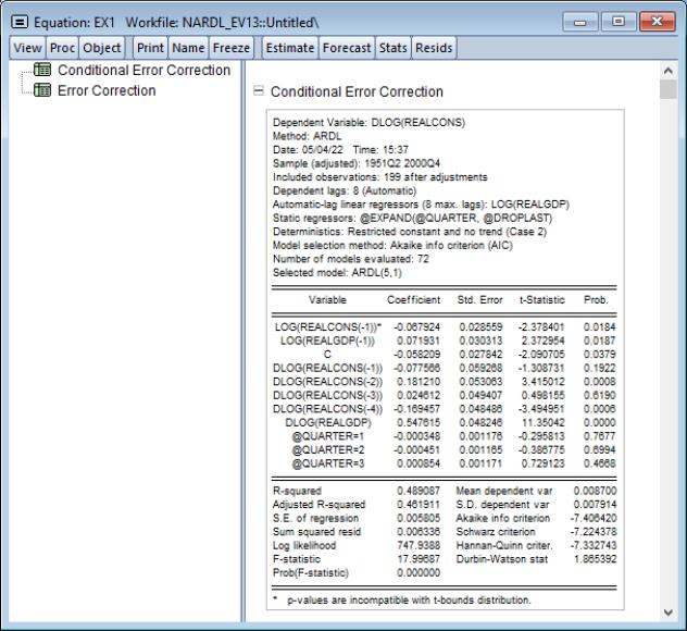
The view displays the estimation results in the error corrections forms. Select from the menu of an estimated ARDL equation. EViews displays a spool with two tables.
The first node in the spool corresponds to the Conditional Error Correction
(CEC) representation (
Equation (29.5) or
Equation (29.17)) of the equation:
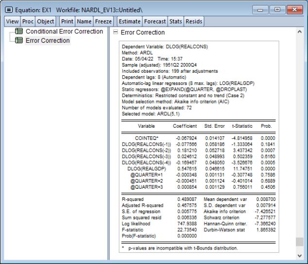
The second node in the spool corresponds to results for the Error Correction (EC) representation of the equation (
Equation (29.10) or
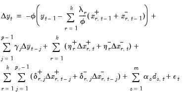
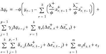
Equation (29.20)), highlighting the speed of adjustment to equilibrium in the cointegrating relationship. The results show the least squares estimates for the equation which employs the equilibrium error correction term in place of the individual cointegrating series:
Here, the error correction term

given by
Equation (29.9) and
Equation (29.19) is included among the regressors and is denoted as “COINTEQ”. The coefficient associated with this regressor is the speed of adjustment to equilibrium in each period. If variables are indeed cointegrated, we typically expect this coefficient to be negative and highly significant.
Note that the name of the lag of the dependent variable and the COINTEQ term in these two tables are always followed by a single asterisk, The single asterisk indicates that the p-value associated with the variable is incompatible with the t-Bounds distribution in Theorem 3.2 in PSS(2001).
The names of other variables may be followed by a double asterisk. A double asterisk indicates that the variable is a dynamic regressor with an optimal lag of zero so that EViews does not include lags and differences of the variables in the specification.
Cointegrating Relation View
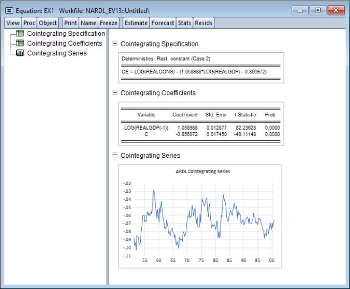
The view displays information about the error correction term

representing the cointegrating relation. Select from the menu of an estimated ARDL equation to display a spool containing two tables and a graph.
• The table shows the assumptions underlying the estimate of the cointegrating relationship, and the equation specification for

.
• The table shows coefficient estimates for the underlying variables inside the cointegrating relationship. These are the

coefficients in
Equation (29.8) and the

and

coefficients in
Equation (29.18).
Bounds Test View
The traditional cointegration tests of Engle (1987), Phillips (1990), or Johansen (1995) require all variables in a VAR system to be

. This requirement not only requires pre-testing for the presence of unit roots in each of the endogenous variables, but is also subject to misclassification.
In contrast, Pesaran (2001) proposes a test for cointegration that is robust to whether variables of interest are

,

, or mutually cointegrated. These
bounds tests are formulated as standard
F-test or Wald tests of parameter significance in the cointegrating relationship of the CEC model
Equation (29.8),
 | (29.28) |
Once the bounds test statistic is computed, the value is compared to two asymptotic critical values corresponding to the polar cases of all variables being

, or all variables being

. When the test statistic is below the lower critical value, we fail to reject the null and conclude that cointegration is not possible. Alternately, when the test statistic is above the upper critical value, we reject the null and conclude that cointegration is possible. In either case, knowledge of the cointegrating rank is not necessary. If the statistic falls between the lower and upper critical values, the test is inconclusive.
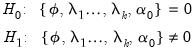
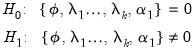
When the hypothesis in
Equation (29.28) is rejected so that cointegration is possible, we proceed to perform a
t-test of significance of the error correction parameter

in
Equation (29.10). As in the case of Augmented Dickey-Fuller unit-root tests, critical values for the test statistic are non-standard. If the null hypothesis of

is not rejected, there is no long run relationship. Alternatively, should we reject

but be unable to reject the sub-hypothesis
, the cointegrating relationship is degenerate. Otherwise, cointegration exists.
When deterministics contribute to the error correction term, they are implicitly projected onto the span of the cointegrating vector. If the ARDL model in
Equation (29.1) includes a constant and a trend, say

and

, the constants and trend coefficients must respect the restrictions implied by the expressions for

and

. These restrictions translate into slight modifications of the null and alternative hypotheses in
Equation (29.28).
We may outline five alternate specifications of the CEC model that are distinguished by whether deterministic terms are included into the error correction term (Pesaran, 2001). The five cases, which closely follow VEC literature (Johansen, 1995), are summarized as follows:
• Case 1 – No constant, no trend: and

which implies that
. There is no change to the
Equation (29.28) bounds test hypothesis.
• Case 2 – Restricted constant and no trend:

and

, so the restrictions

and

are assumed to hold:
 | (29.29) |
• Case 3 – Unrestricted constant and no trend:

and

, and the restrictions

and

are assumed to hold. There is no change to the
Equation (29.28) bounds test hypothesis.
• Case 4 – Unrestricted constant and restricted trend:

and

, and the restrictions

and

are assumed hold:
 | (29.30) |
• Case 5 – Unrestricted constant and unrestricted trend:

and

and the restrictions

and

are assumed hold. There is no change to the
Equation (29.28) bounds test hypothesis.
To perform the bounds test, click on . The results are presented in a spool. Below the table of long run coefficient estimates are two additional tables, respectively titled as the

-Bounds Test and the

-Bounds Test.
These tables respectively display the

- and

- statistics along with their associated I(0) (lower) and I(1) (upper) critical value bounds for the null hypotheses of no levels relationship between the dependent variable and the regressors in the CEC model. The critical values are provided for significance levels 10%, 5%, 2.5%, and 1%, respectively. The

-Bounds test in particular is a parameter significance test on the lagged value of the dependent variable. Since the distribution of this test is non-standard, the

-value provided in the regression output of the CEC regression is not compatible with this distribution, although the

-statistic is valid. Accordingly, any inference must be conducted using the

-Bounds test critical values provided.
We also mention here that the

- critical value tables now present the critical values computed under an asymptotic regime (sample size equal to 1000) and referenced from PSS(2001), in addition to providing critical values for finite sample regimes (sample sizes running from 30 to 80 in increments of 5) and referenced from Narayan (2005).
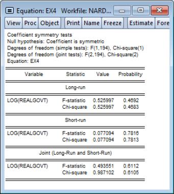
Symmetry Test View
Recall that the NARDL CEC representation in
Equation (29.20) is quite general and can accommodate asymmetries in different combinations of short and long-run dynamics. In particular, consider the following two sets of symmetry restrictions:
1. Long-run Symmetry: Restricts
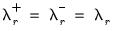
for all

so that the CEC reduces to
 | (29.31) |
2. Short-run Symmetry: Restricts
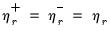
and
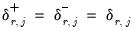
for

and
, so the CEC reduces to
 | (29.32) |
Imposing either set of restrictions leads to one of the previous two representations. Imposing both restrictions reduces the NARDL CEC representation to the classical ARDL CEC representation in
Equation (29.8)And of course, it is possible to generate even more complex dynamics by imposing symmetry on other subsets of the long-run and short run regressors.
Naturally, one can test for symmetry formally by performing the usual
t-test or
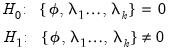
F-test of parameter equality. For example, testing for symmetry for a specific long-run (LR) variable, say

, is equivalent to the following hypothesis:
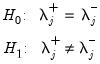 | (29.33) |
To perform the symmetry test, select from the menu of a nonlinear asymmetric NARDL equation:
Dynamic Multipliers View
Dynamic multipliers (DM) are a familiar concept which measures the marginal contribution of an explanatory variable to the dependent variable. A natural extension of the concept for time series analysis is the idea of
cumulative dynamic multipliers (CDM). This is the cumulative sum of dynamic multipliers at each point in time, starting with a point in time

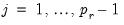
and running through

for horizon length

.
Background
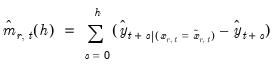
For standard ARDL models, CDMs are defined for each long-run distributed-lag variable using the partial derivatives:
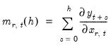 | (29.34) |
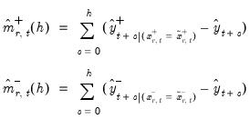
For nonlinear ARDL models, CDMs are derived for any long-run asymmetric distributed-lag variables using the partial derivatives s for both the positive and negative partial sum regressors:
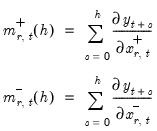 | (29.35) |
where
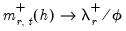
and
. We may employ the absolute difference between the two derivatives,
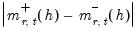
, as a measure of nonlinearity.
Following convention, we will measure the adjustments of the dependent variable

to unit shocks in the respective regressors,

, or

and

. Conceptually, for a given regressor, a single positive unitary shock is introduced at

, where

is the end of the estimation sample, holding all other regressors constant. The dynamic evolution of the dependent variable is then computed from

to

and compared to baseline dynamic forecasts.
The adjusted in-sample dynamic forecasts are given by first shocking the

value of the target regressor,
 | (29.36) |
and
 | (29.37) |
for shocks

, and then forming the
dynamic forecasts of

from

to

using the estimated equation, actual regressors, and the substituted modified regressor:
• in the symmetric case we substitute in

for the initial value

and use this value to obtain the forecasts
• in the asymmetric case, we compute two forecasts using the actual regressors with a single substitution; first substituting in

for

to obtain the forecasts
, and then substituting in

for

to obtain the forecasts
Then the discrete dynamic multipliers are given by the accumulated differences between the modified, and the original dynamic forecasts:
 | (29.38) |
and
 | (29.39) |
where

is the unmodified in-sample dynamic forecast from the estimated equation.
There are two conventions for defining the unit shocks

in
Equation (29.36) and
Equation (29.37):
• the
Dynamic Multiplier Evolution convention, sets
. Here, the unit changes in
Equation (29.37) produce an increase in the cumulated symmetric and positive differences and a
reduction in the cumulated negative difference.
• the
Shock Evolution convention, sets

and

. Here, we define the impulses so that there is an increase in the cumulated symmetric and positive differences, and an
increase in the cumulated negative difference.
While the dynamic multiplier evolution framework is reasonable from a technical perspective, it is not ideal if we wish to study the properties of the models under parallel unit increases in the absolute amount of positive and negative asymmetry, as in when determining whether an increase in positive asymmetry has the same effect as an increase in negative asymmetry.
Dynamic Multiplier View
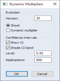
To display CDM graphs for each of the explanatory variables, click on EViews will open a dialog containing display and computation settings:
• You may enter the horizon length  (number of periods to compute the multipliers) in the
 edit field. The multiplier graphs will be produced for the period from

to

where

is the end of the estimation sample.
• You may select whether to display a CDM graph based on the evolution of shocks or on the dynamic multiplier. This distinction does not matter for symmetric models, but the graph types do differ in their asymmetric negative response curves.
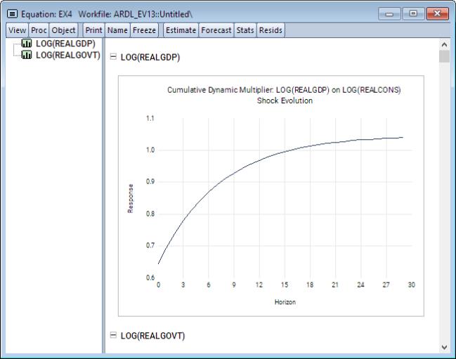
The shock evolution CDM graph displays the response to a one unit positive change in the symmetric and positive asymmetric cumulated differences, and the response to a one unit negative change in cumulated differences in the negative asymmetric case. Note that in this case, the graphswill converge to the theoretical cumulative dynamic multiplier long-run values.
The dynamic multiplier CDM graph shows the response to a one unit positive change in symmetric and asymmetric cumulated differences, but in contrast to shock evolution, models an “improvement” producing a one unit positive increase (reduction of one unit of negative change) in the negative cumulative differences.
• For NARDL models, you will be offered the opportunity to display confidence intervals for the computed absolute difference between the positive and negative components for a given regressor. CIs are not available for linear ARDL specifications.
• You may check the to display the CIs, and to display the CIs as bands instead of lines. The edit field controls the size of the CI, and the governs how many replications to use in resampling for computing the CI.
Click on to continue. EViews will open a spool view, with each node in the spool containing the CDM graph corresponding to one of the explanatory variables.
For symmetric linear models, each shock evolution graph contains a CDM. In case of the dynamic multiplier evolution curves, there is an additional dashed horizontal line denoting the long-run value.
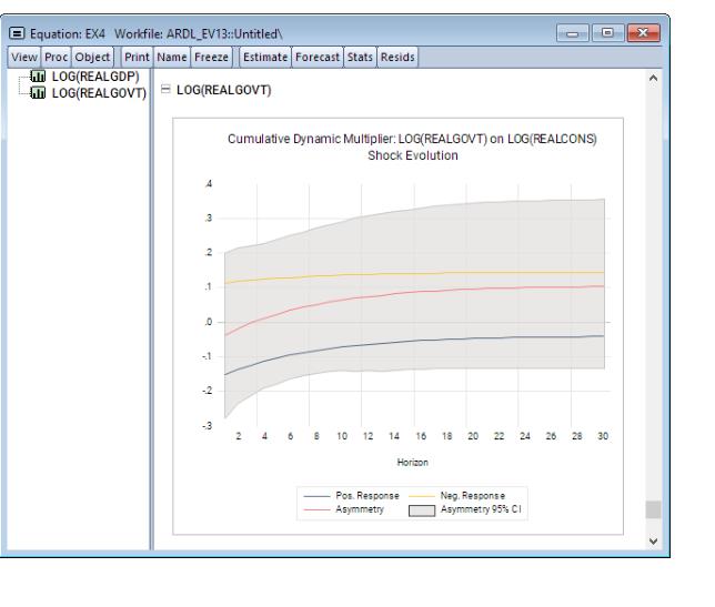
For asymmetric nonlinear models, each graph will show the positive and negative responses, along with a line showing the absolute value of the difference between the two, and if requested, a CI for the absolute difference:
ARDL Equation Procs
Most of the procs for an ARDL equation are familiar from other estimation methods. Some procs require a bit of additional discussion.
Make Regressor Group Proc
Displays a group containing the regressors for the estimated specification.
For all models, this group will include the specified or selected number of lags of the dependent variable and dynamic regressors, along with any fixed variables.
For the asymmetric ARDL specifications, the group will also contain the regressors formed using the cumulative positive and negative functions @cumdp and @cumdn, and the accumulation differences @dcumdp and @dcumdn.
Make Cointegrating Relationship Proc
The proc makes a series in the workfile containing the cointegrating series, which contains

(
Equation (29.9) or
Equation (29.19)) for every observation in the estimation sample.
 (
Equation (29.9) or
Equation (29.19)) for every observation in the estimation sample.
(
Equation (29.9) or
Equation (29.19)) for every observation in the estimation sample.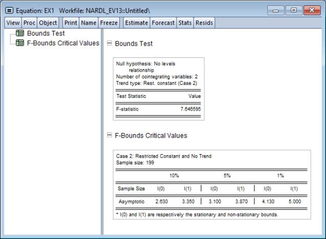
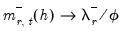
 . Note that as
  ,
,  .
.