Examples
We demonstrate ARDL estimation using a dataset from Greene (2008, page 685). This dataset consists of a number of quarterly US macroeconomic variables between 1950 and 2000. The data are in the workfile “Ardl_ex.WF1”
Example 1: Symmetric ARDL (Automatic Lag Selection)
Here we start with a classical (symmetric) ARDL model using the log of real consumption as the dependent variable, and the log of real GDP as a single regressor (along with a constant). We can open the data with the following EViews command:
wfopen http://www.stern.nyu.edu/~wgreene/Text/Edition7/TableF5-2.txt
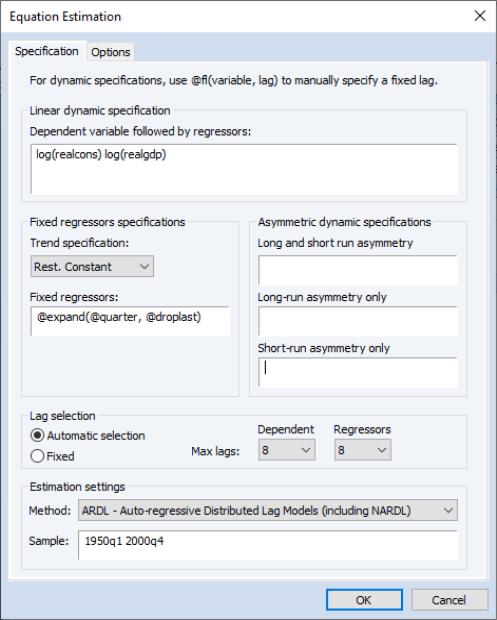
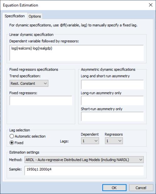
Next, bring up the estimation dialog and ensure that the Method dropdown under the Estimation specification is Least-squares. Next, enter
log(realcons) log(realgdp)
into the Linear dynamic specification. Select Automatic selection with a maximum of 8 lags (two years) for both the dependent variable and dynamic regressors. We will also include a full set of quarterly dummies as fixed regressors. In particular, we will restrict the constant to the cointegrating relationship, whereas the remaining quarterly dummies are treated as short-run regressors. To achieve this, we include the long-run constant by choosing Rest. Constant from the Trend specification dropdown, and write
@expand(@quarter, @droplast)
into the Fixed regressors box.
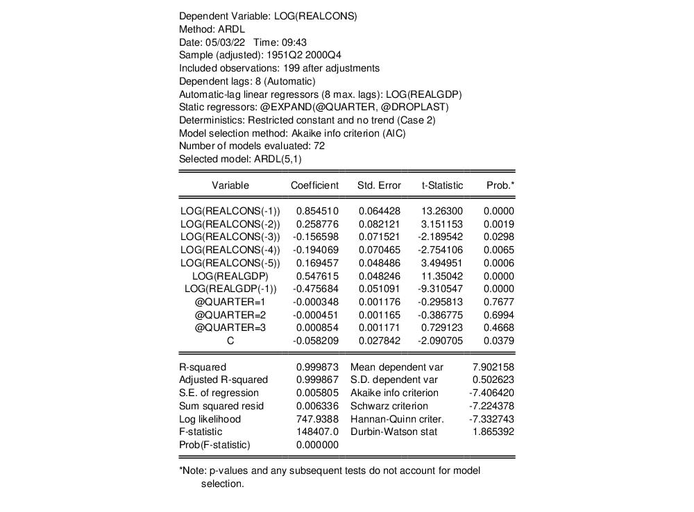
We do not make any changes to the tab, leaving all settings at their default value. The results are shown below:
The first part of the output gives a summary of the settings used during estimation. Here we see that automatic selection (using the Akaike Information Criterion) was used with a maximum of 8 lags of both the dependent variable and the regressor. Out of the 72 models evaluated, the procedure has selected an ARDL(5,1) model - 5 lags of the dependent variable, LOG(REALCONS), and a single lag (along with the level value) of LOG(REALGDP).
The rest of the output is standard least squares output for the selected model. Note that each of the regressors (with the exception of the quarterly dummies) is significant, and that the coefficient on the one period lag of the dependent variable, LOG(REALCONS), is quite high, at 0.85.
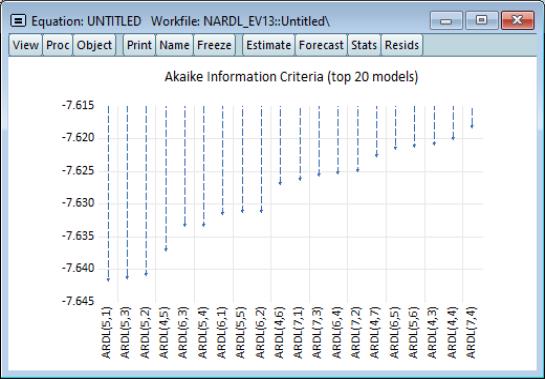
To view the relative superiority of the selected model against alternatives, we click on View/Model Selection Summary/Criteria Graph to view a graph of the AIC of the top twenty models.
The selected ARDL(5,1) model was only slightly better than an ARDL(5,3) model, which was in turn only slightly better than an ARDL(5,2). It is notable that the top three models all use five lags of the dependent variable.
Example 2: Symmetric ARDL(3,3)
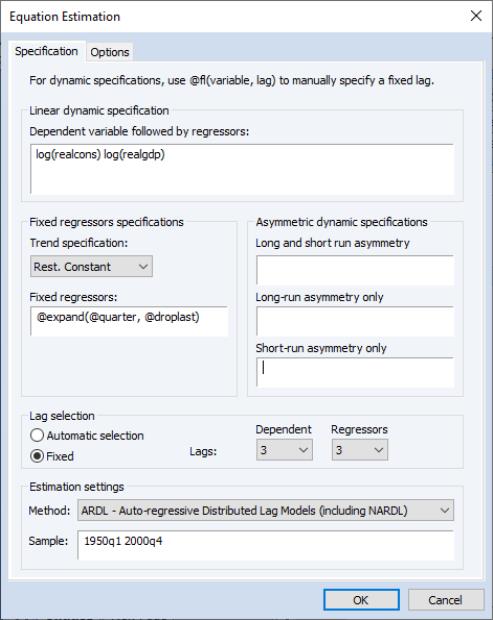
Rather than using automatic selection to choose the best model, Greene (Example 20.4) also analyzes
these data with a fixed ARDL(3,3) model. We can replicate this by pressing the Estimate button to bring up the estimation dialog again. Again, ensure that the Method dropdown under the Estimation specification is Least-squares. This time, we change the number of lags on both dependent and regressors to 3, and then select the Fixed radio button to switch off automatic lag selection.
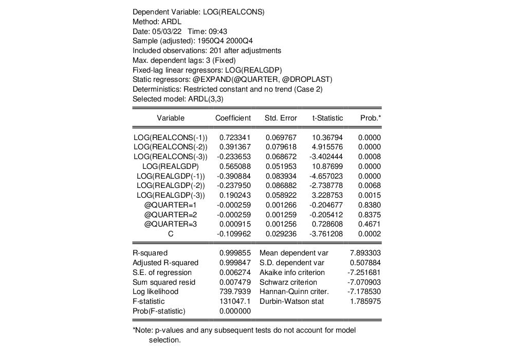
The results of this estimation are:
The one-period lag on the dependent variable remains high, at 0.72, and again all coefficients are significant (with the exception of the dummies).
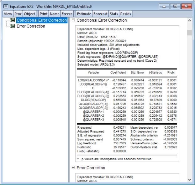
We may examine the CEC and EC forms of the estimates by selecting . EViews will display long-run output in the form of a spool with two tables showing the regression results, and the results. The first table displays the estimation results in the CEC form:
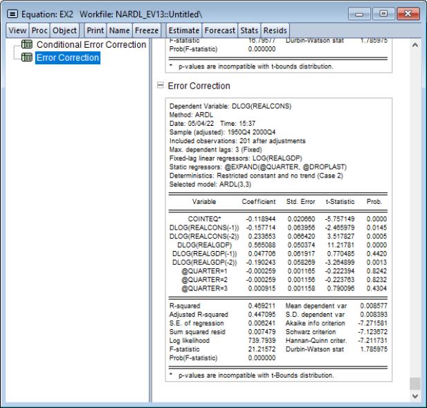
The EC results, which are displayed click on the node, show that the speed of adjustment coefficient is negative (-11.89) and statistically significant,
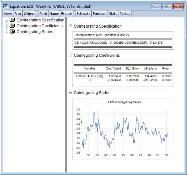
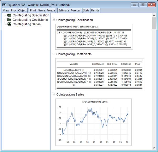
Clicking on shows the specification and coefficient results for the cointegrating relationship:
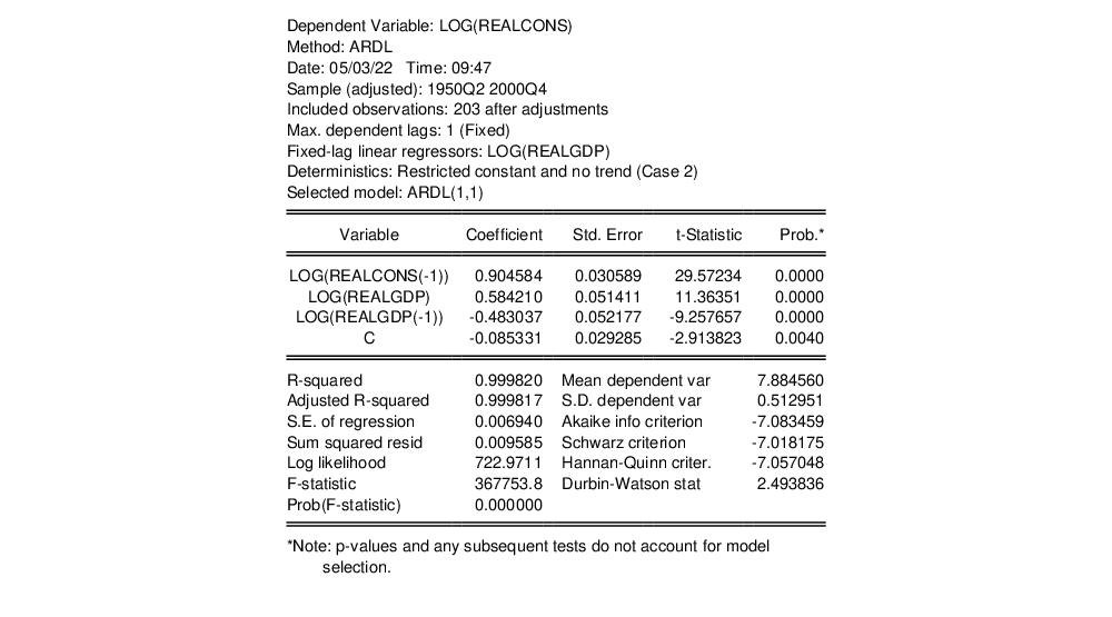
Example 3: Symmetric ARDL(1,1)
As a final symmetric ARDL example, we will consider Greene’s Example 20.5 which estimates an ARDL(1,1) model. Again, from the ARDL equation object, bring up the estimation dialog by clicking on the Estimate button and change the number of lags to 1 for both dependent and regressors, remove the quarterly dummies, and then click OK.
The results of this estimation are:
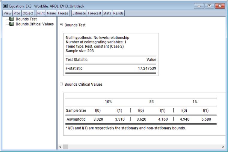
Following estimation, we can perform bounds test for cointegration by clicking on View/ARDL Diagnostics/Bounds Test to bring up the cointegrating relationship view
The bounds statistic is 17.25. We can compare this to the critical values listed in the second table. Clearly the statistic is larger than the I(1) bound critical value at all significance levels. We therefore reject the null hypothesis of no levels relationship and conclude that LOG(REALGDP) are LOG(REALCONS) cointegrated.
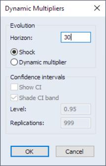
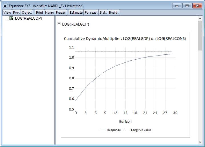
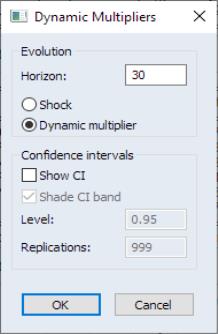
We can also evaluate the dynamic multiplier of LOG(REALGDP) on LOG(REALCONS). To do so, click on View/ARDL Diagnostics/Dynamic Multiplier Graph... to bring up the dynamic multiplier dialog.
Put 30 as the horizon length and click on OK. Note that confidence interval settings are not available for purely symmetric ARDL models.
Here we see that LOG(REALGDP) approaches its long-run value of 1.06 as the horizon length increases. Moreover, it does so at a diminishing pace.
Example 4: Asymmetric ARDL(1,1,1)
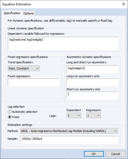
Here we will continue from the previous example, but consider the NARDL(1,1,1) model of LOG(REALCONS) on LOG(REALGDP) and LOG(REALGOVT). In particular, we will treat LOG(REALGOVT) as an asymmetric variable which is asymmetric in both the short-run and the long-run. To estimate this model, bring up the estimation dialog by clicking on the Estimate button. Next, type
log(reagovt)
into the Long-run and short-run edit field under the Asymmetric dynamic specification group, and click on OK.
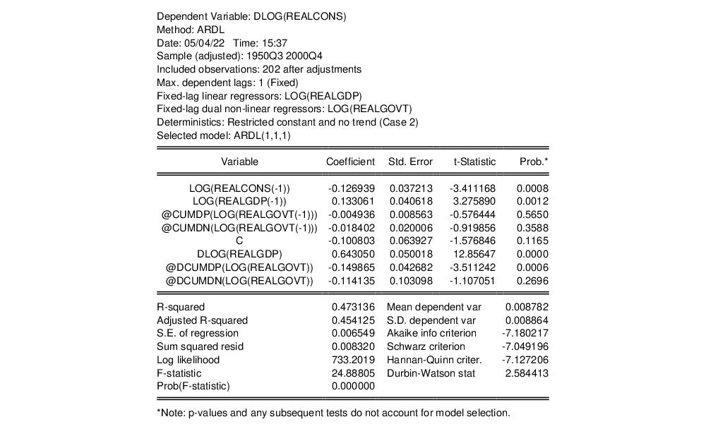
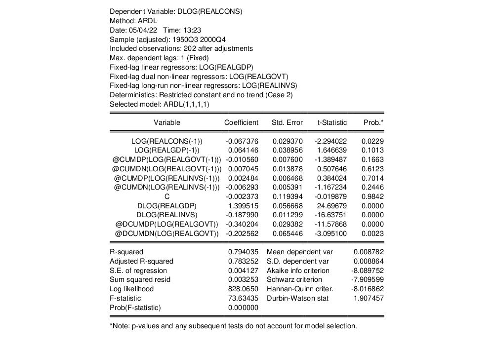
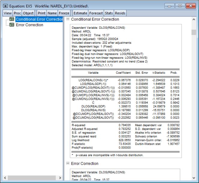
The results of this estimation are:
Notice that LOG(REALGOVT) is now split into two variables corresponding to the positive and negative cumulative sums, prefaced respectively as POS_ and NEG_.
NOTE: It is extremely important to notice that unlike the case of purely symmetric ARDL models which display the estimation of
Equation (29.1) as the default output, the default estimation output for NARDL models is always the CEC equation
Equation (29.17). This is due to the fact that partial asymmetry (as in Example 5 below) is specified in the context of a NARDL CEC model in
Equation (29.17), and CEC models naturally distinguish between long- and short- variables. Accordingly, the conversion of partial asymmetry from
Equation (29.17) into
Equation (29.16) becomes difficult and sometimes leads to unidentifiability.
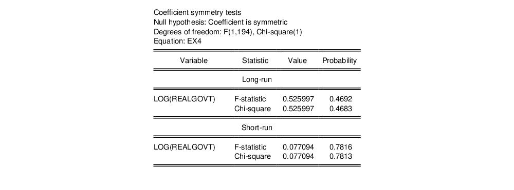
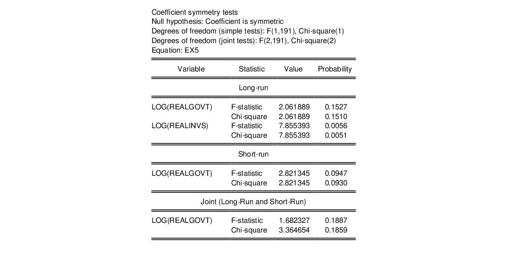
We can also test whether the asymmetric assumption on LOG(REALGOVT) is valid by testing each asymmetric variable for symmetry. To do so, click on View/ARDL Diagnostics/Symmetry Test.
The result is a table for symmetry in both the long-run and short-run scope. As the null hypothesis of these test is symmetry, we will reject the null hypothesis in the long-run scope, but fail to reject it in the short-run scope.
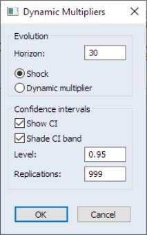
Let’s also derive the dynamic multiplier curves. Click on View/ARDL Diagnostics/Dynamic Multiplier Graph... to bring up the dynamic multiplier dialog.
Notice that the options for confidence intervals is now available. This is because dynamic multiplier CIs are derived for the absolute difference in paths resulting from the positive and negative asymmetric components of a given regressor. Moreover, CIs are derived by resampling methods, and therefore the Replications textbox governs how many replications are used to derive a CI.
To proceed, put 30 as the horizon length and leave everything at else at its default values. Click on OK.
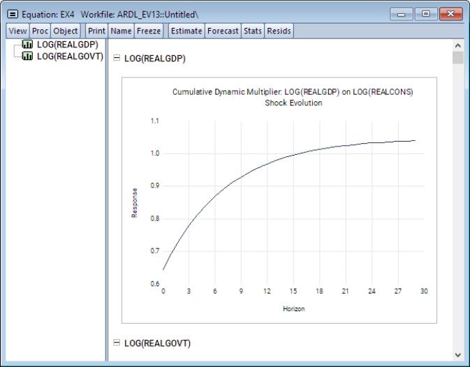
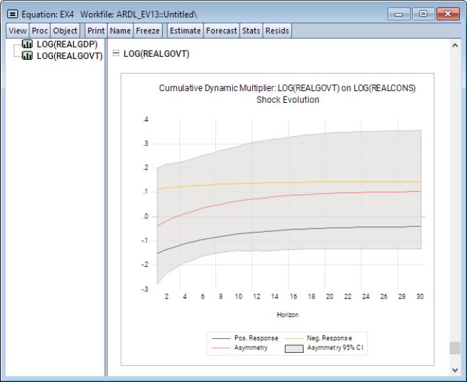
Notice that all paths approach their long-run values, which are indicated by dashed horizontal lines in the plots. Furthermore, since LOG(REALGOVT) is asymmetric in both the long-run and short-run, we expect the dynamic multiplier curves to diverge in both the long-run and short-run. This is evidenced by the fact that the absolute difference between these paths (indicated as the red curve) never approaches zero. Furthermore, notice the gray shaded area which displays the desired confidence interval the absolute asymmetry.
Example 5: Asymmetric ARDL(1,1,1,1)
Continuing with the previous example, we will now add a partially symmetric variable to the list of distributed-lag regressors. In particular, we will treat REALINVS – real investments – as a variable which is asymmetric in the long-run, but symmetric in the short run. Again, bring up the estimation dialog by clicking on the Estimate button. Next, type
log(realinvs)
into the Long-run only edit field, and press OK.
The results of this estimation are:
Note that in contrast to LOG(REALGOVT) which is asymmetric in both the long-run and shortrun, LOG(REALINVS) is split into its positive and negative cumulative sums in the long-run, but remains symmetric in the short-run. We can study the CEC form further by clicking on Views/ARDL Diagnostics/Conditional Error Correction (Long Run) Form.
We see here that both LOG(REALGOVT) and LOG(REALINVS) now enter the cointegrating relationship.
We can also conduct a symmetry test by proceeding to View/ARDL Diagnostics/Symmetry Test.
Here, since LOG(REALGOVT) is a fully asymmetric variable, it is tested for symmetry among both the long-run and short-run regressors. In particular, we fail to reject symmetry for LOG(REALGOVT) in both the long-run and short-run scopes. Nevertheless, since LOG(REALINVS) is asymmetric in the long-run and symmetric in the short-run, the test for asymmetry is only available in the long-run. Here in fact, we will reject the null of symmetry at any meaningful p-value.
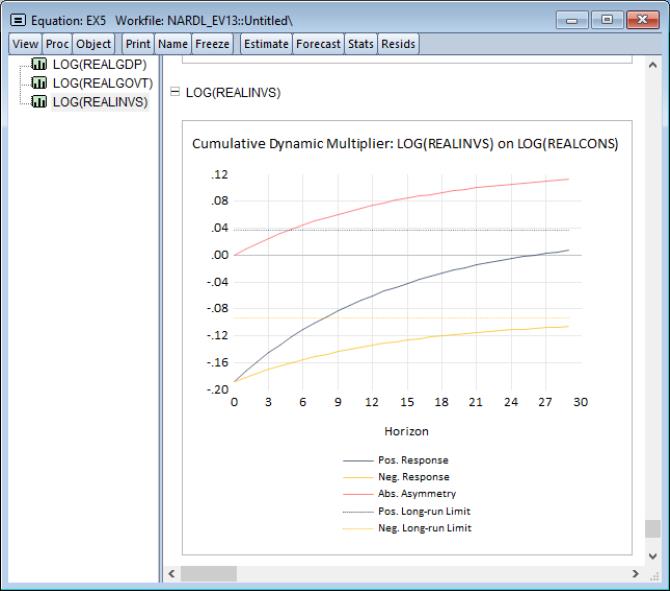
To derive the dynamic multiplier curves we again click on View/ARDL Diagnostics/Dynamic Multiplier Graph... to bring up the dynamic multiplier dialog.
Here we will generate the curves without displaying confidence intervals. As before, put 30 as the horizon length, click on the Show CI checkbox to deselect it, click on OK.
Of particular interest here is the final curve associated with LOG(REALINVS). Recall that the latter is asymmetric in the long-run, but is symmetric in the short-run. This is also clearly seen by noting the absolute asymmetry curve which starts off at zero, but the then diverges in the long-run.
Example 6: Asymmetric ARDL(1,1,1,1,1)
Adding further to the previous example, we now add another partially symmetric variable to the list of distributed-lag regressors. In particular, we will treat LOG(TBILRATE) – treasury bill rate – as a variable which is asymmetric in the short-run, but symmetric in the long-run. Again, bring up the estimation dialog by clicking on the Estimate button. Next, type
log(tbilrate)
into the Short-run only textbox, and press OK.
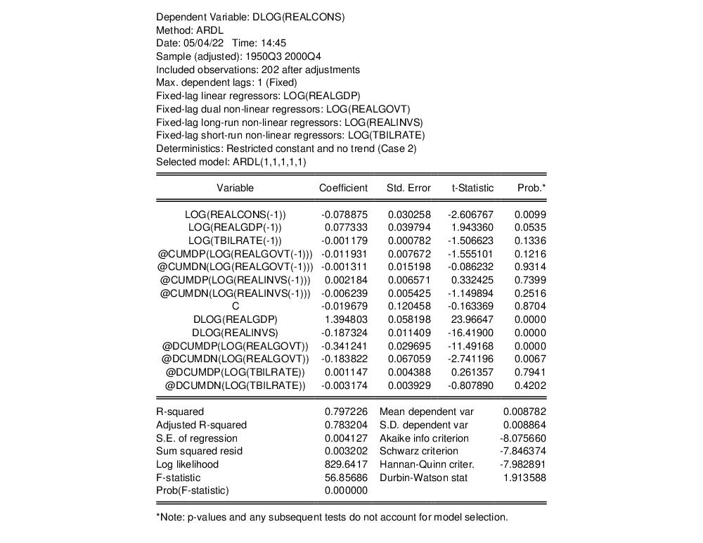
The estimation results are:
Note that LOG(TBILRATE) now appears among the long-run regressors, and that @DCUMDP(TBILRATE) and @DCUMDN(TBILRATE), the asymmetric components of LOG(TBILRATE), only appear among the short-run regressors.
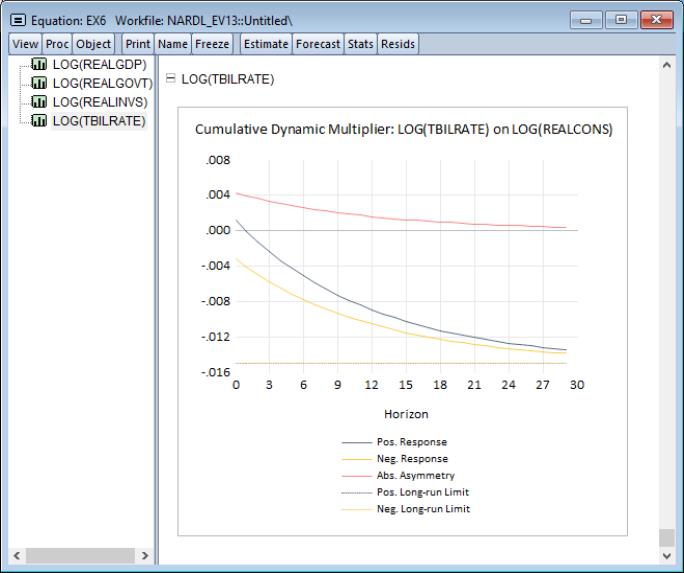
Let’s derive the dynamic multipliers for the constituent regressors here as well. Proceed to View/ARDL Diagnostics/Dynamic Multiplier Graph... to bring up the dynamic multiplier dialog. Put 30 as the horizon length and deselect the Show CI checkbox. Click on OK.
As in the previous example, our focus is on the final curve. In particular, LOG(TBILRATE) is asymmetric in the short-run, but symmetric in the long-run. Accordingly, absolute asymmetry is above zero at the start of the evolution, but then settles to zero as we approach the long-run.
Example 7: Quantile ARDL(1,1)
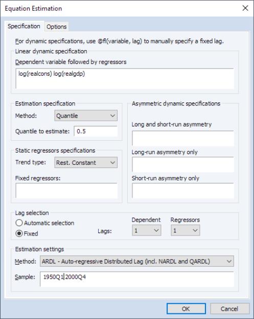
In this example, we will estimate a simple quantile ARDL model at the median quantile. To estimate, bring up the estimation dialog and type
log(realcons) log(realgdp)
into the Linear dynamic specification. Since we’re estimating a QARDL model, select Quantile under the Method dropdown in the Estimation specification group. Lastly, leave the Quantile to estimate at its default 0.5 (median) value, and press OK.
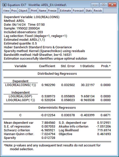
Estimation results are:
The output is analogous to the classical ARDL model output. In particular, the output produces the inter-temporal ARDL form, estimated using quantile regression. Moreover, the summary above the results table provides additional information relevant to quantile estimation, such as sparsity and bandwidth specifications.
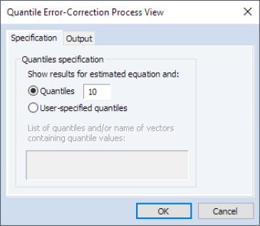
We can now visualize the error-correction quantile process. Click on View/ARDL Diagnostics/Quantile Error-Correction Results Process.... This produces a dialog where we can specify which quantiles we’d like to consider in deriving the process.
We can leave the Specification tab at its default, which will produce the process for 10 equally spaced quantile values. Alternatively, if a set of specific quantiles is desired, they can be specified by clicking on the User-specified quantiles and supplying a space-delimited list in the textbox.
If you’d like to write the process (quantiles, coefficients, and covariances) to the workfile, you can click on the Output tab and provide output names for the quantile vector and the coefficient and covariance matrices. Note that since this view derives the process for both the CEC and the EC forms, output objects will be differentiated by an automatic suffix ("_CEC" or "_EC") appended to the output names provided for the coefficient and covariance matrices.
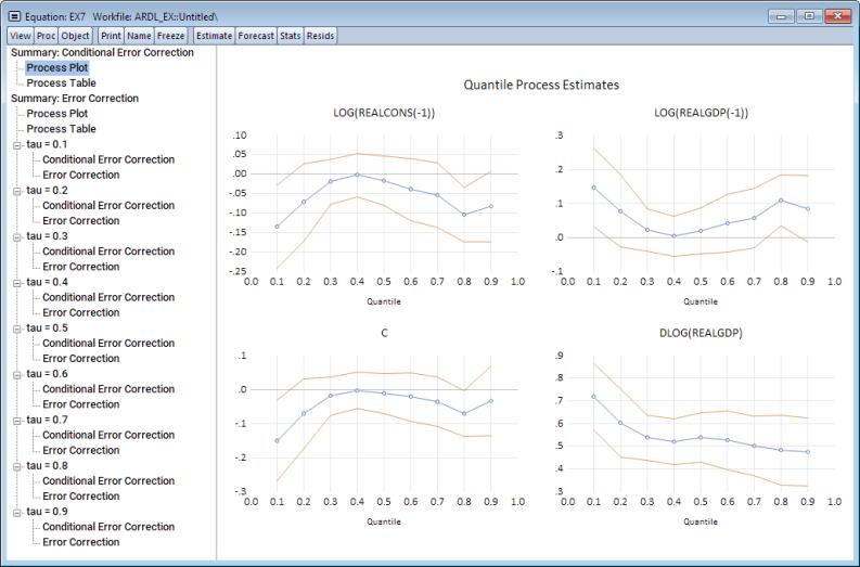
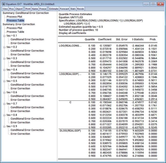
The default output here is a plot of the quantile process of the coefficients associated with the CEC form.
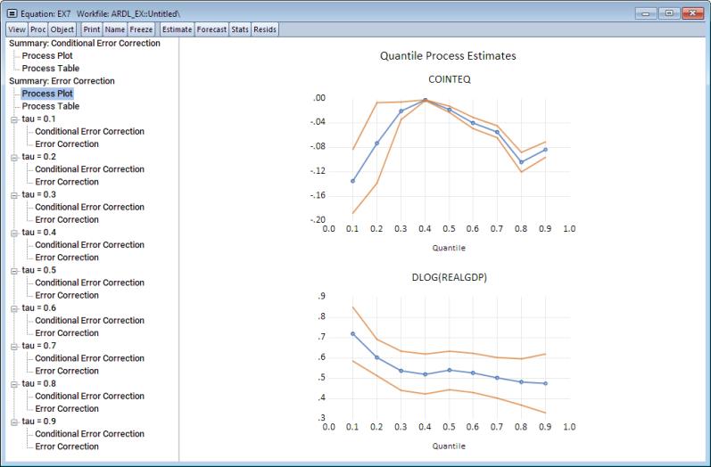
To display the quantile process for the coefficients of the EC form, click on the Process Plot node beneath the Summary: Error-Correction Process parent in the navigation tree to the left.
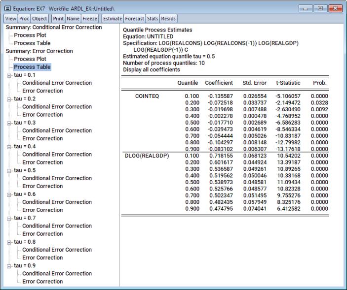
If you prefer, you can also display the table version of these plots. Simply click on Process Table nodes in the navigation tree to the left.
If you prefer to inspect the CEC or EC estimation tables at any specific quantile value, click on the Conditional Error Correction or Error Correction nodes beneath the appropriate quantile value (tau) parents in the navigation tree.
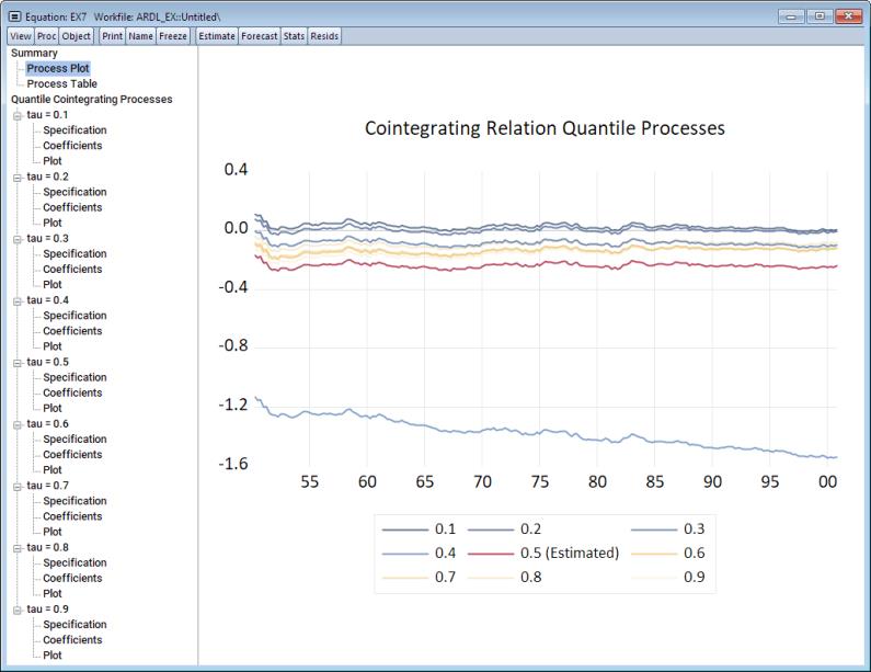
We can produce similar outputs for the quantile process associated with the cointegrating relation. To do so, navigate to View/ARDL Diagnostics/Quantile Cointegrating Relation Process. A dialog similar to the quantile error-correction process appears. We’ll stick with the defaults so click on OK.
The output produced is a set of cointegrating relation series at each quantile value superimposed on a single plot, with additional options to generate the corresponding table, or even look at the process coefficients and plots at each individual quantile value.
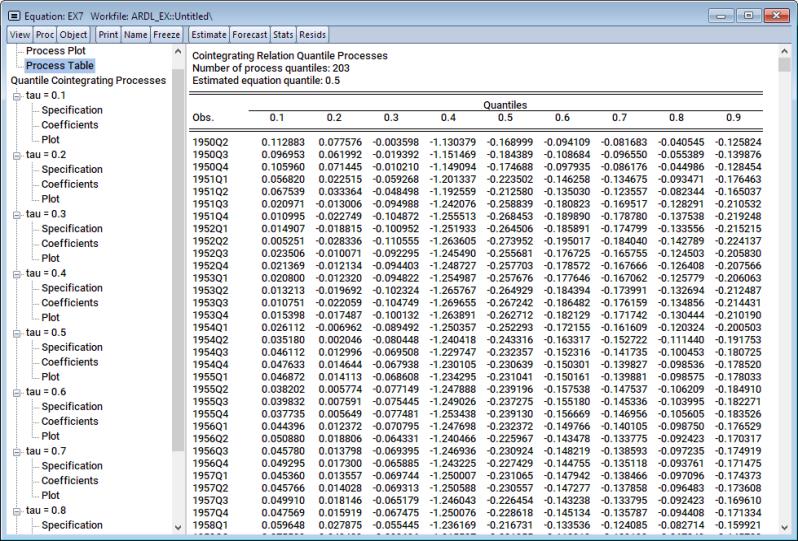
If instead you’d like to inspect the plot as table, click on the Process Table node beneath the Summary parent in the navigation tree.
Alternatively, you can inspect the specification, long-run coefficients, or even the cointegrating relation plot at any specific quantile value. Simply click on the Specification, Coefficients, or Plot nodes beneath the appropriate quantile value (tau) parents in the navigation tree.