EViews Help: Post-Estimation Procedures

Most of the post-estimation views and procs available in standard VARs are also available for Bayesian VARs. However, with a few exceptions, these procedures simply take the estimate of the mean or covariance of the posterior distributions and applies these to classical techniques as if they were classical point estimates. To make this explicit, the view and proc menu items are labeled “Classical…”

Some procedures have been modified to allow a more Bayesian approach. These procedures make the distinction between the posterior residual moments (estimated moments of the posterior distribution and the empirical residual moments (residual moments calculated using the classical approach:

using Equation (47.4)).

The residuals view (View/Residuals) now offers two choices for the residual covariance display: Empirical Covariance Matrix (the covariance of the empirical residuals) and Posterior Covariance Matrix (the covariance estimated from the posterior distribution).

To produce impulse response graphs and tables, you may select View/Impulse Response... As with other VAR estimation methods, the first two tabs of the dialog (Display and Impulse Definition) will prompt you to select which impulses and responses to display in graph or table form, and to define the impulses you wish to produce.

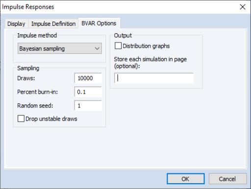
The impulse response dialog for Bayesian VARs has an additional BVAR Options tab that contains Bayesian Specific settings:

The Impulse method dropdown menu selects the method for computing the impulses:

• Classical – posterior res cov. performs classical impulse response analysis where the impulses are calculated based upon the posterior residual covariance.

• Classical – empirical res cov. performs classical impulses response analysis where the impulses are calculated based upon the empirical residual covariance.

If Bayesian sampling is selected as the impulse method, the Sampling and Output options allow you to customize the sampling and store output:

• The Drop unstable draws checkbox determines whether EViews will throw out and re-sample any draw which results in VAR coefficients that produce an unstable VAR. Note that checking this box may severely increase the time taken to produce the impulses if the posterior probability that the VAR is stable is low.

• The Distribution graphs check box will produce kernel-distribution plots of the draws for each variable pair and each period of the responses.

• The Store each simulation in page edit field allows you to enter the name of a page in which to store each individual draw of the sampler. If a name is entered into this box, a new page with that name will be created in the workfile, structured as a panel with one dimension representing the number of response periods, and the other corresponding to the number of posterior draws. EViews will create a series for each variable pair in the new page.

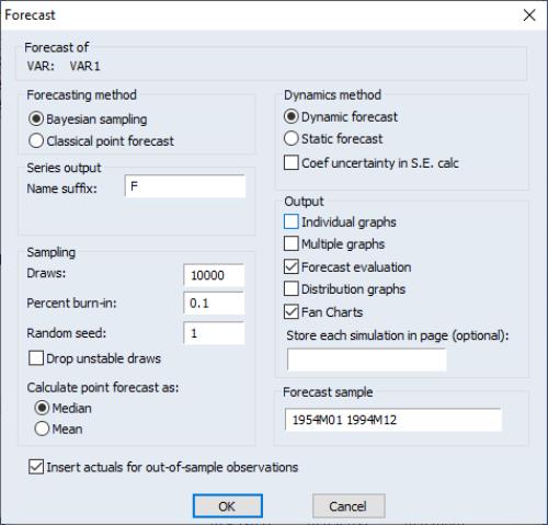
Selection Proc/Forecast... displays the forecast dialog which offers a choice between Bayesian or classical forecasting:

By default, EViews will produce forecasts using Bayesian sampling, but you may select the Classical point forecast radio button to use the estimated coefficients to produce a point forecast.

If Bayesian sampling is selected, the Sampling and Output options allow you to customize the sampling and store output as in Bayesian impulse response calculation:

• The Distribution graphs check box will produce kernel-distribution plots of the draws for each variable pair and each period of the responses.

• The Store each simulation in page edit field allows you to enter the name of a page in which to store each individual draw of the sampler. If a name is entered into this box, a new page with that name will be created in the workfile, structured as a panel with one dimension representing then umber of response periods, and the other corresponding to the number of non-burned in sample draws. EViews will create a series for each variable pair in the new page.

The Bayesian sampling approach to either impulse responses or forecasting from the VAR will differ depending upon the type of prior that was used during estimation.

For priors that have a closed-form solution for the posterior: Litterman, normal-flat, normal-Wishart, Sims-Zha normal-flat and Sims-Zha normal-Wishart, although the posterior distribution of the VAR coefficients and covariances can be calculated without simulation, the posterior distribution of non-linear functions of the coefficients and covariance will still require calculation through Monte-Carlo integration simulations.

Following Koop and Korobilis 2010, EViews performs this integration by pulling a draw of Sigma from its posterior distribution, and then using that draw of Sigma to pull a draw of alpha from its conditional posterior distribution, and, in the case of forecasting, pull a draw of the forecast errors. These draws are then used to compute an impulse or forecast. This process is repeated many times, and the overall mean of the responses or forecasts is computed.

A closed form solution for the posterior distributions of the independent normal-Wishart prior does not exist, so estimation is performed using a Gibbs sampler. Consequently, calculation of impulses or forecasts from the VAR also require use of a Gibbs sampler. Specifically, the sampler is run identically as to during estimation, but at each draw of alpha and Sigma during the sampler, an impulse response or forecast is computed from the draws. Note that the same random number generator seed used during estimation will be used for draws of alpha and Sigma. For forecasting the seed specified on the forecast dialog is used for draws of the residuals at each stage of the sampler.

The nature of the Giannone, Lenza and Primiceri prior requires the use of a Metropolis-Hastings sampler for characterizing the posterior, and consequently for sampling impulse responses or forecasts.

EViews allows you to take draws from the posterior distributions of either the coefficients or the residual covariance matrix by selecting Proc/Draw from Coefficient Posterior or Proc/Draw from Residual Covariance Posterior.

For all prior types apart from independent normal-Wishart, this procedure involves simply taking IID draws from the posterior distribution. For the independent normal-Wishart prior, a Gibbs sampler is employed.