An Example
We illustrate the basic features of the factor object by analyzing a subset of the classic Holzinger and Swineford (1939) data, consisting of measures on 24 psychological tests for 145 Chicago area children attending the Grant-White school (Gorsuch, 1983). A large number of authors have used these data for illustrating various features of factor analysis. The raw data are provided in the EViews workfile “Holzinger24.WF1”. We will work with a subset consisting of seven of the 24 variables: VISUAL (visual perception), CUBES (spatial relations), PARAGRAPH (paragraph comprehension), SENTENCE (sentence completion), WORDM (word meaning), PAPER1 (paper shapes), and FLAGS1 (lozenge shapes).
(As noted by Gorsuch (1983, p. 12), the raw data and the published correlations do not match; for example, the data in “Holzinger24.WF1” produces correlations that differ from those reported in Table 7.4 of Harman (1976). Here, we will assume that the raw data are correct; later, we will show you how to work directly with the Harman reported correlation matrix.)
Specification and Estimation
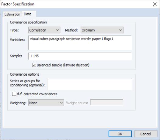
Since we have previously created a group object G7 containing the seven series of interest, double click on G7 to open the group and select . EViews will open the main factor analysis specification dialog.
When the factor object created in this fashion, EViews will pre-define a specification based on the series in the group. You may click on the tab to see the pre-filled settings. Here, we see that EViews has entered in the names of the seven series in G7.
The remaining default settings instruct EViews to calculate an ordinary (Pearson) correlation for all of the series in the group using a balanced version of the workfile sample. You may change these as desired, but for now we will use these settings.
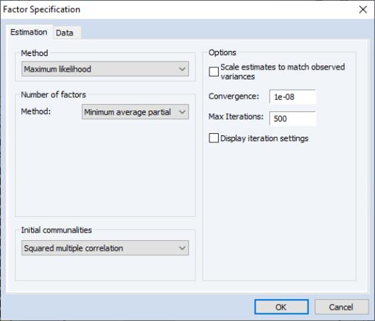
Next, click on the tab to see the main factor analysis settings. The settings may be divided into three main categories: (extraction), , and . In addition, the section on the right of the dialog may be used to control miscellaneous settings.
By default, EViews will estimate a factor specification using maximum likelihood. The number of factors will be selected using Velicer’s minimum average partial (MAP) method, and the starting values for the communalities will be taken from the squared multiple correlations (SMCs). We will use the default settings for our example so you may click on to continue.
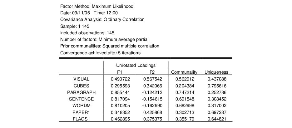
EViews estimates the model and displays the results view. Here, we see the top portion of the main results. The heading information provides basic information about the settings used in estimation, and basic status information. We see that the estimation used all 145 observations in the workfile, and converged after five iterations.
Below the heading is a section displaying the estimates of the unrotated orthogonal loadings, communalities, and uniqueness estimates obtained from estimation.
We first see that Velicer’s MAP method has retained two factors, labeled “F1” and “F2”. A brief examination of the unrotated loadings indicates that PARAGRAPH, SENTENCE and WORDM load on the first factor, while VISUAL, CUES, PAPER1, and FLAGS1 load on the second factor. We therefore might reasonably label the first factor as a measure of verbal ability and the second factor as an indicator of spatial ability. We will return to this interpretation shortly.
To the right of the loadings are communality and uniqueness estimates which apportion the diagonals of the correlation matrix into common (explained) and individual (unexplained) components. The communalities are obtained by computing the
row norms of the loadings matrix, while the uniquenesses are obtained directly from the ML estimation algorithm. We see, for example, that 56% (
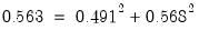
) of the correlation for the VISUAL variable and 69% (
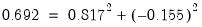
) of the SENTENCE correlation are accounted for by the two common factors.
The next section provides summary information on the total variance and proportion of
common variance accounted for by each of the factors, derived by taking column norms of the loadings matrix. First, we note that the variance accounted for by the two factors is 3.55, which is close to 51% (

) of the total variance (sum of the diagonals of the correlation matrix). Furthermore, we see that the first factor F1 accounts for 77% (

) of the
common variance and the second factor F2 accounts for the remaining 23% (

).
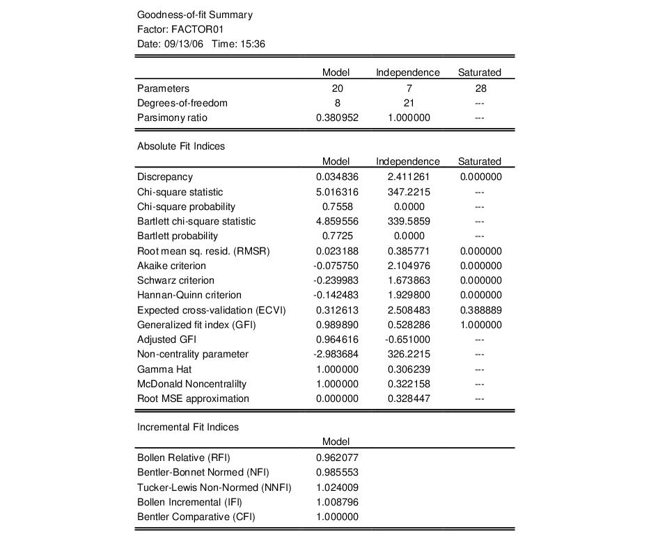
The bottom portion of the output shows basic goodness-of-fit information for the estimated specification. The first column displays the discrepancy function, number of parameters, and degrees-of-freedom (against the saturated model) for the estimated specification For this extraction method (ML), EViews also displays the chi-square goodness-of-fit test and Bartlett adjusted version of the test. Both versions of the test have p-values of over 0.75, indicating that two factors adequately explain the variation in the data.
For purposes of comparison, EViews also presents results for the independence (no factor) model which show that a model with no factors does not adequately model the variances.
Basic Diagnostic Views
Once we have estimated our factor specification we may examine a variety of diagnostics. First, we will examine a variety of goodness-of-fit statistics and indexes by selecting from the factor menu.
As you can see, EViews computes a large number of absolute and relative fit measures. In addition to the discrepancy, chi-square and Bartlett chi-square statistics seen previously, EViews computes scaled information criteria, expected cross-validation indices, generalized fit indices, as well as various measures based on estimates of noncentrality. Also presented are incremental fit indices which compare the fit of the estimated model against the independence model (see
“Model Evaluation” for discussion).
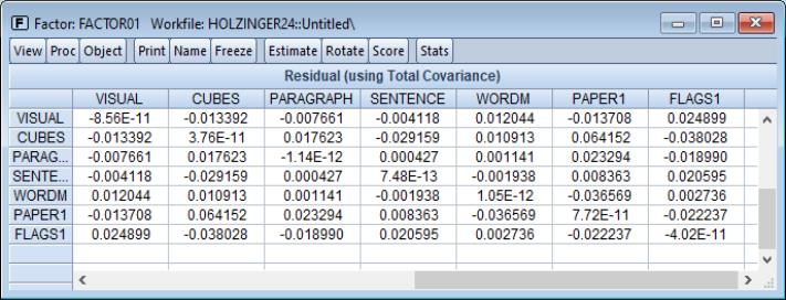
In addition, you may examine various matrices associated with the estimation procedure. You may examine the computed correlation matrix, various reduced and fitted matrices, and a variety of residual matrices. For example, you may view the residual variance matrix by selecting .
Note that the diagonal elements of the residual matrix are (near) zero since we have subtracted off the total fitted covariance (which includes the uniquenesses). To replace the (near) zero diagonals with the uniqueness estimates, select instead .
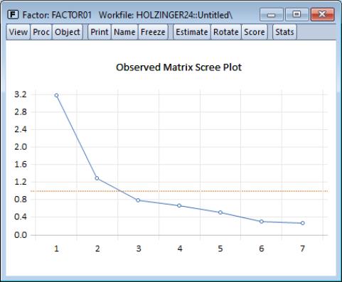
You may examine eigenvalues of relevant matrices using the eigenvalue view. EViews allows you to compute eigenvalues for a variety of matrices and display the results in tabular or graphical form, but for the moment we will simply produce a scree plot for the observed correlation matrix. Select and change the to .
Click on to accept the settings. EViews will display the scree plot for the data, along with a line indicating the average eigenvalue.
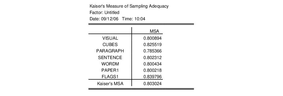
To examine the Kaiser Measure of Sampling Adequacy, select . The top portion of the display shows the individual measures and the overall of MSA (0.803) which falls in the category deemed by Kaiser to be “meritorious”.
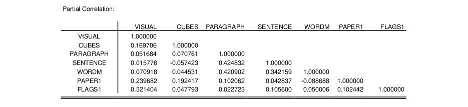
The bottom portion of the display shows the matrix of partial correlations:
Each cell of this matrix contains the partial correlation for the two variables, controlling for the remaining variables.
Factor Rotation
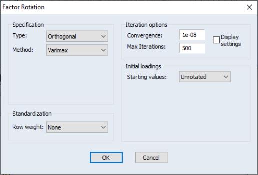
Factor rotation may be used to simplify the factor structure and to ease the interpretation of factors. For this example, we will consider one orthogonal and one oblique rotation. To perform a factor rotation, click on the button on the factor toolbar or select from the main factor menu.
The factor rotation dialog is used to specify the rotation method, row weighting, iteration control, and choice of initial loadings. We begin by accepting the defaults which rotate the initial loadings using orthogonal Varimax. EViews will perform the rotation and display the results.
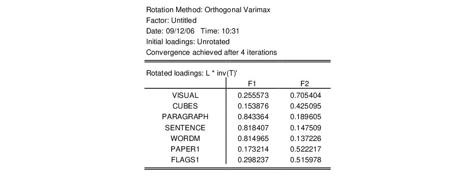
The top portion of the displayed output provides information about the rotation and shows the rotated loadings.
As with the unrotated loadings, the variables PARAGRAPH, SENTENCE, and WORDM load on the first factor while VISUAL, CUBES, PAPER1, and FLAGS1 load on the second factor.
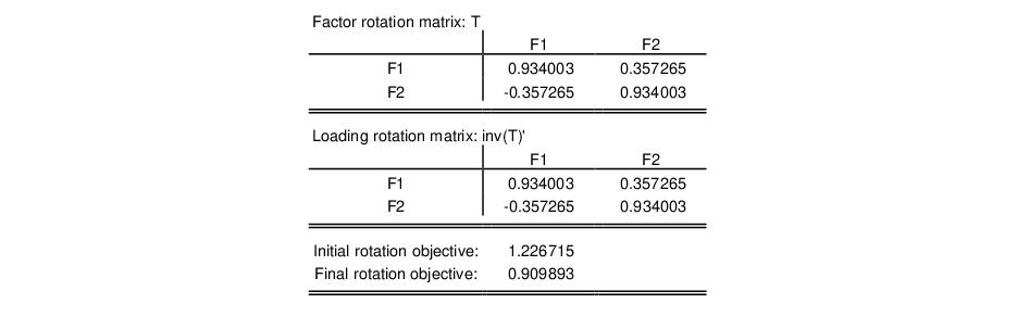
The remaining sections of the output display the rotated factor correlation, initial rotation matrix, the rotation matrices applied to the factors and loadings, and objective functions for the rotations. In this case, The factor correlation and initial rotation matrices are identity matrices since we are performing an orthogonal rotation from the unrotated loadings. The remaining results are presented below:
Note that the factor rotation and loading rotation matrices are identical since we are performing an orthogonal rotation.
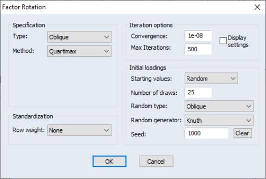
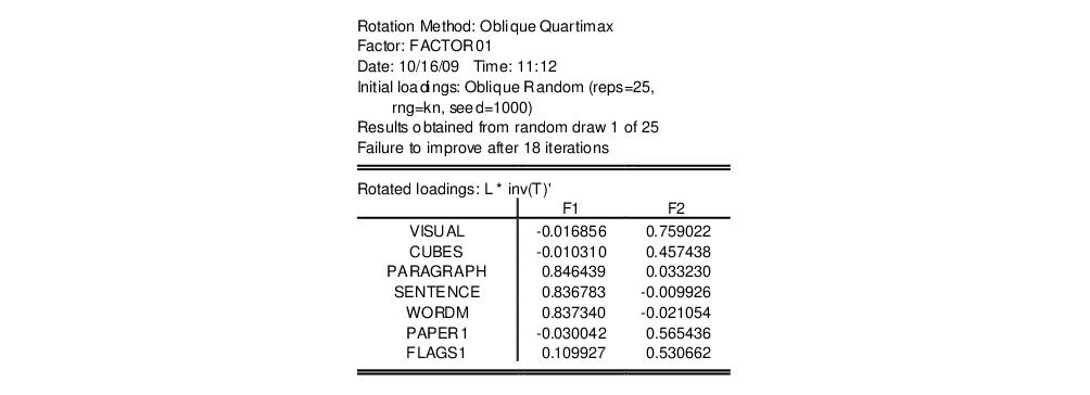
Perhaps more interesting are the results for an oblique rotation. To replace the Varimax results with an oblique Quartimax/Quartimin rotation, select and change the dropdown to , and select . We will make a few other changes in the dialog. We will use random orthogonal rotations as starting values for our rotation, so that under , you should select . Set the random generator options as depicted and change the convergence tolerance to 1e-06. By default, EViews will perform 25 oblique rotations using random orthogonal rotation matrices as the starting values, and will select the results with the smallest objective function value. Click on to accept these settings.
The top portion of the results shows information on the rotation method and initial loadings. Just below the header are the rotated loadings. Note that the relative importance of the VISUAL, CUBES, PAPER1, and FLAGS1 loadings on the second factor is somewhat more apparent for the oblique factors.
The rotated factor correlation is:
with the large off-diagonal element indicating that the orthogonality factor restriction was very much binding.
The rotation matrices and objective functions are given by:
Note that in the absence of orthogonality, the factor rotation and loading rotation matrices differ.
Once a rotation has been performed, the last set of rotated loadings will be available to all routines that use loadings. For example, to visualize the factor loadings, select to bring up the loadings graph dialog.
Here you will provide indices for the factor loadings you wish to display. Since there are only two factors, EViews has prefilled the dialog with “1 2” indicating that it will plot the second factor against the first factor.
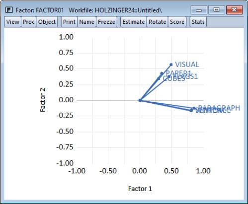
By default, EViews will use the rotated loadings if available; note the checkbox allowing you to use the unrotated loadings. Check this box and click on to display the unrotated loadings graph.
As is customary, the loadings are displayed as lines from the origin to the points labeled with the variable name. Here we see visual evidence of our previous interpretation: the variables cluster naturally into two groups (factors), with factor 1 representing verbal ability (PARAGRAPH, SENTENCE, WORDM), and factor 2 representing spatial ability (VISUAL, PAPER1, FLAGS1, CUBES).
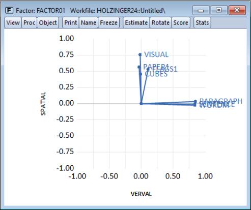
Before displaying the oblique Quartimax rotated loadings, we will apply this labeling to the factors. Select and enter “Verbal” and “Spatial” in the dialog. EViews will subsequently label the factors using the specified names instead of the generic labels “Factor 1” and “Factor 2.”
Now, let us display the graph of the rotated loadings. Click on and simply click on to accept the defaults. EViews displays the rotated loadings graph. Note the clear separation between the sets of tests.
Factor Scores
The factors used to explain the covariance structure of the observed data are unobserved, but may be estimated from the rotated or unrotated loadings and observable data.
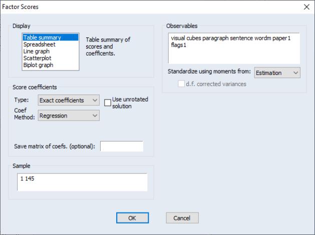
Click on to bring up the factor score dialog. As you can see, there are several ways to estimate the factors and several views of the results. For now, we will focus on displaying a summary of the factor score regression estimates, and in producing a biplot of the scores and loadings.
The default method of producing scores is to use exact coefficients from Thurstone’s regression method, and to apply these coefficients to the observables data used in factor extraction.
In our example, EViews will prefill the sample and observables information; all we need to do is to select our setting, and the method for computing coefficients. Selecting , EViews produces output describing the score coefficient estimation.
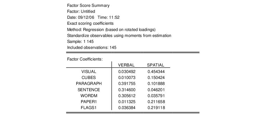
The top portion of the output summarizes the factor score coefficient estimation settings and displays the factor coefficients used in computing scores:
We see that the VERBAL score for an individual is computed as a linear combination of the centered data for VISUAL, CUBES, etc., with weights given by the first column of coefficients (0.03, 0.01, etc.).
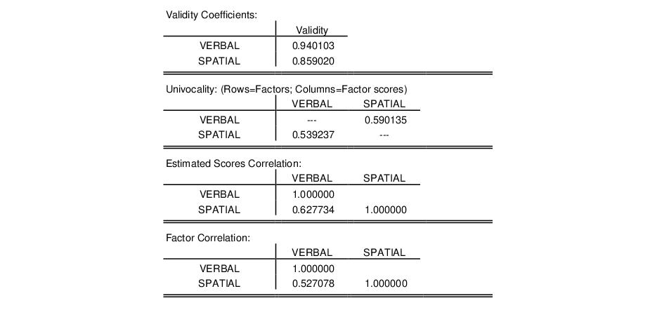
The next section contains the factor indeterminacy indices:
The indeterminacy indices show that the correlation between the estimated factors and the variables is high; the multiple correlation for the first factor well over 0.90, while the correlation for the second factor is around 0.85. The minimum correlation indices are also reasonable, suggesting that alternative factor score solutions are highly correlated. At a minimum, the correlation between two different measures of the SPATIAL factors will be nearly 0.50.
The following sections report the validity coefficients, the off-diagonal elements of the univocality matrix, and for comparison purposes, the theoretical factor correlation matrix and estimated scores correlation:
The validity coefficients are both in excess of the Gorsuch (1983) recommended 0.80, and close to the stricter target of 0.90 advocated for using the estimated scores as replacements for the original variables.
The univocality matrix reports the correlations between the factors and the factor scores, which should be similar to the corresponding elements of the factor correlation matrix. Comparing results, we see that univocality correlation of 0.539 between the SPATIAL factor and the VERBAL estimated scores is close to the population correlation value of 0.527. The correlation between the VERBAL factor and the SPATIAL estimated score is somewhat higher, 0.590, but still close to the population correlation.
Similarly, the estimated scores correlation matrix should be close to the population factor correlation matrix. The off-diagonal values generally match, though as is often the case, the factor score correlation of 0.627 is a bit higher than the population value of 0.527.
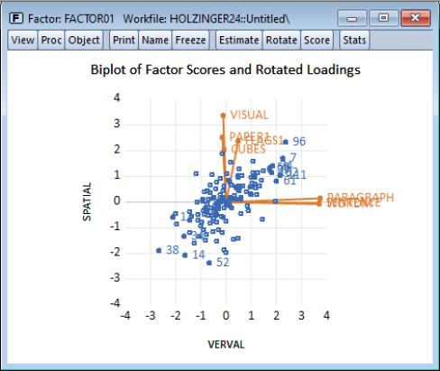
To display a biplot of using these scores, select and select in the list box.
The positive correlation between the VERBAL and SPATIAL scores is obvious. The outliers show that individual 96 scores high and individual 38 low on both spatial and verbal ability, while individual 52 scores poorly on spatial relative to verbal ability.
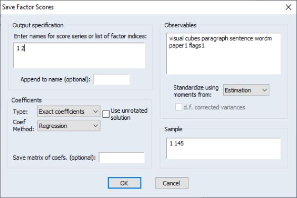
To save scores to the workfile, select and fill out the dialog. The procedure dialog differs from the view dialog only in the section. Here, you should enter a list of scores to be saved or a list of indices for the scores. Since we have previously named our factors, we may specify the indices “1 2” and click on . EViews will open an untitled group containing the results saved in the series VERBAL and SPATIAL.