Creating a Factor Object
Factor analysis in EViews is carried out using a factor object. You may create and specify the factor object in a number of ways. The easiest methods are:
• Select from the workfile menu, choose , and enter the specification in the dialog.
• Highlight several series, right-click, select and enter the specification in the dialog.
• Open an existing group object, select and enter the specification in the dialog.
You may also use the commands factor or factest to create and specify your factor object.
Specifying the Model
There are two distinct parts of a factor object specification. The first part of the specification describes which measure of association or dispersion, typically a correlation or covariance matrix, EViews should fit using the factor model. The second part of the specification defines the properties of the factor model.
The dispersion measure of interest is specified using the tab of the dialog, and the factor model is defined using the tab. The following sections describe these settings in detail.
Data Specification
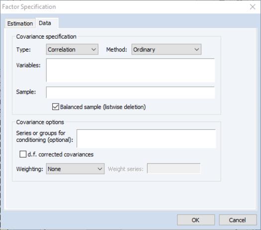
The first item in the tab is the dropdown menu, which is used to specify whether you wish to compute a or matrix from the series data, or to provide a containing a previously computed measure of association.
Covariance Specification
Here we see the dialog layout when or is selected.
Most of these fields should be familiar from the Covariance Analysis view of a group. Additional details on all of these settings may be found in
“Covariance Analysis”.
Method
You may use the dropdown to specify the calculation method: ordinary Pearson covariances, uncentered covariances, Spearman rank-order covariances, and Kendall’s tau measures of association.
Note that the computation of factor scores (
“Scoring”) is not supported for factor models fit to Spearman or Kendall’s tau measures. If you wish to compute scores for measures based on these methods you may, however, estimate a factor model fit to a user-specified matrix.
Variables
You should enter the list of series or groups containing series that you wish to employ for analysis.
(Note that when you create your factor object from a group object or a set of highlighted series, EViews assumes that you wish to compute a measure of association from the specified series and will initialize the edit field using the series names.)
Sample
You should specify a sample of observations and indicate whether you wish to balance the sample. By default, EViews will perform listwise deletion when it encounters missing values. This option is ignored when performing partial analysis (which may only be computed for balanced samples).
Partialing
Partial covariances or correlations may be computed for each pair of analysis variables by entering a list of conditioning variables in the edit field.
Computation of factor scores is not supported for models fit to partial covariances or correlations. To compute scores for measures in this setting you may, however, estimate a factor model fit to a user-specified matrix.
Weighting
When you specify a weighting method, you will be prompted to enter the name of a weight series. There are five different weight choices: frequency, variance, standard deviation, scaled variance, and scaled standard deviation.
Degrees-of-Freedom Correction
You may choose to compute covariances using the maximum likelihood estimator or the degree-of-freedom corrected formula. By default, EViews computes ML estimates (no d.f. correction) of the covariances. Note that this choice may be relevant even if you will be working with a correlation matrix since standardized data may be used when constructing factor scores.
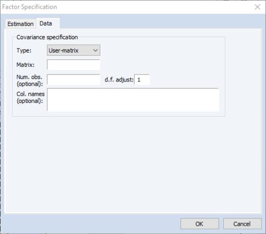
User-matrix Specification
in the Type dropdown, the dialog changes, prompting you for the name of the matrix and optional information for the number of observations, the degrees-of-freedom adjustment, and column names.
• You should specify the name of an EViews matrix object containing the measure of association to be fit. The matrix should be square and symmetric, though it need not be a sym matrix object.
• You may enter a scalar value for the number of observations, or a matrix containing the pairwise numbers of observations. A number of results will not be computed if a number of observations is not provided. If the pairwise number of observations is not constant, EViews will use the minimum number of observations when computing statistics.
• Column names may be provided for labeling results. If not provided, variables will be labeled “V1”, “V2”, etc. You need not provide names for all columns; the generic names will be replaced with the specified names in the order they are provided.
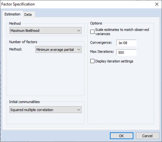
Estimation Specification
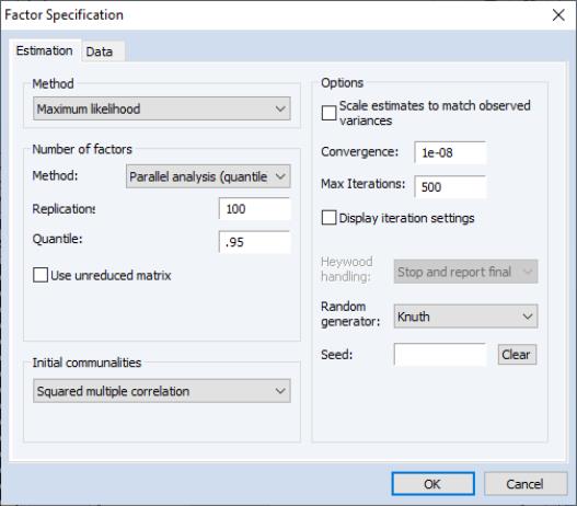
The main estimation settings are displayed when you click on the tab of the dialog. There are four sections in the dialog allowing you to control the method, number of factors, initial communalities, and other options. We describe each in turn.
Method
In the dropdown menu, you should select your estimation method. EViews supports estimation using , , , , , and methods.
Depending on the method, different settings may appear in the section to the right.
Number of Factors
EViews supports a variety of methods for selecting the number of factors. By default, EViews uses Velicer’s (1976) minimum average partial method (MAP). Simulation evidence suggests that MAP (along with parallel analysis) is more accurate than more commonly used methods such as Kaiser-Guttman (Zwick and Velicer, 1986). See
“Number of Factors” for a brief summary of the various methods.
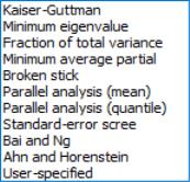
You may change the default by selecting an alternative method from the dropdown menu. The dialog may change to prompt you for additional input:
• The method allows you to employ a modified Kaiser-Guttman rule that uses a different threshold. Simply enter your threshold in the edit field.
• If you select , EViews will prompt you to enter the target threshold.
• If you select either or from the dropdown menu, the dialog page will change to provide you with a number of additional options.
In the sections, EViews will prompt you for the number of simulations to run, and, where appropriate, the quantile of the empirical distribution to use for comparison.
By default, EViews compares the eigenvalues of the reduced matrix against simulated eigenvalues. This approach is in the spirit of Humphreys and Ilgen (1969), who use the SMC reduced matrix. If you wish to use the eigenvalues of the original (unreduced) matrix, simply check .
The section of the page provides options for the random number generator and the random seed. While the dropdown should be self-explanatory, the field requires some discussion.
By default, the first time that you estimate a given factor model, the edit field will be blank; you may provide your own integer value, if desired. If an initial seed is not provided, EViews will randomly select a seed value at estimation time. The value of this initial seed will be saved with the factor object so that by default, subsequent estimation will employ the same seed. If you wish to use a different value, simply enter a new value in the edit field or press the button to have EViews draw a new random seed value.
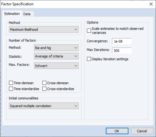
• If you select either or from the dropdown menu, the dialog page will offer different options.
The dialog settings are described in detail in
“Bai and Ng” and
“Ahn and Horenstein” .
Initial Communalities
Initial estimates of the common variances are required for most estimation methods. For iterative methods like ML and GLS, the initial communalities are simply starting values for the estimation of uniquenesses. For principal factor estimation, the initial communalities are fundamental to the construction of the estimates (see
“Principal Factors”).
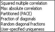
By default, EViews will compute SMC based estimates of the communalities. You may select a different method using the dropdown menu. Most of the methods should be self-explanatory; a few require additional comment.
• performs a non-iterative PACE estimation of the factor model and uses the fitted estimates of the common variances. The number of factors used is taken from the main estimation settings.
• The setting instructs EViews to use a different random fraction of each diagonal element of the original dispersion matrix.
• The values will be subtracted from the original variances to form communality estimates. You will specify the name of the vector containing the uniquenesses in the edit field. By default, EViews will look at the first elements of the C coefficient vector for uniqueness values.
To facilitate the use of this option, EViews will place the estimated uniqueness values in the coefficient vector C. In addition, you may use the equation data member @unique to access the estimated uniqueness from a named factor object.
See
“Communality Estimation” for additional discussion.
Estimation Options
We have already seen the iteration control and random number options that are available for various estimation and number of factor methods. The remaining options concern the scaling of results and the handling of Heywood cases.
Scaling
Some estimation methods guarantee that the sums of the uniqueness estimates and the estimated communalities equal the diagonal dispersion matrix elements; for example, principal factors models compute the uniqueness estimates as the residual after accounting for the estimated communalities.
In other cases, the uniqueness and loadings are both estimated directly. In these settings, it is possible for the sum of the components to differ substantively from the original variances.
You can enforce the adding up condition by checking the box. If this option is selected, EViews will automatically adjust your uniqueness and loadings estimates so the sum of the unique and common variances matches the diagonals of the dispersion matrix. Note that when scaling has been applied, the reported uniquenesses and loadings will differ from those used to compute fit statistics; the main estimation output will indicate the presence of scaled results.
Heywood Case Handling
In the course of iterating principal factor estimation, one may encounter estimated communalities which implies that at least one unique variance is less than zero; these situations are referred to as Heywood cases.
When you encounter a Heywood case in EViews, there are several approaches that you may take. By default, EViews will stop iterating and report the final set of estimates (), along with a warning that the results may be inappropriate. Alternately, you may instruct EViews to report the previous iteration’s results (, to set the results to zero and continue (), or to ignore the negative unique variance and continue ().