Two-stage Least Squares
Two-stage least squares (TSLS) is a special case of instrumental variables regression. As the name suggests, there are two distinct stages in two-stage least squares. In the first stage, TSLS finds the portions of the endogenous and exogenous variables that can be attributed to the instruments. This stage involves estimating an OLS regression of each variable in the model on the set of instruments. The second stage is a regression of the original equation, with all of the variables replaced by the fitted values from the first-stage regressions. The coefficients of this regression are the TSLS estimates.
You need not worry about the separate stages of TSLS since EViews will estimate both stages simultaneously using instrumental variables techniques. More formally, let

be the matrix of instruments, and let

and

be the dependent and explanatory variables. The linear TSLS objective function is given by:
 | (23.1) |
Then the coefficients computed in two-stage least squares are given by,
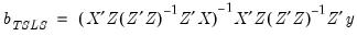 | (23.2) |
and the standard estimated covariance matrix of these coefficients may be computed using:
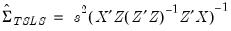 | (23.3) |
where

is the estimated residual variance (square of the standard error of the regression). If desired,

may be replaced by the non-d.f. corrected estimator. Note also that EViews offers both White and HAC covariance matrix options for two-stage least squares.
Estimating TSLS in EViews
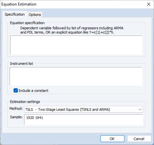
To estimate an equation using Two-stage Least Squares, open the equation specification box by choosing or Choose TSLS from the Method: dropdown menu and the dialog will change to include an edit window where you will list the instruments.
Alternately, type the tsls keyword in the command window and hit ENTER.
In the edit box, specify your dependent variable and independent variables and enter a list of instruments in the edit box.
There are a few things to keep in mind as you enter your instruments:
• In order to calculate TSLS estimates, your specification must satisfy the order condition for identification, which says that there must be at least as many instruments as there are coefficients in your equation. There is an additional rank condition which must also be satisfied. See Davidson and MacKinnon (1993) and Johnston and DiNardo (1997) for additional discussion.
• For econometric reasons that we will not pursue here, any right-hand side variables that are not correlated with the disturbances should be included as instruments.
• EViews will, by default, add a constant to the instrument list. If you do not wish a constant to be added to the instrument list, the check box should be unchecked.
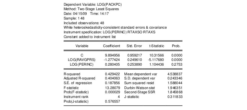
To illustrate the estimation of two-stage least squares, we use an example from Stock and Watson 2007 (p. 438), which estimates the demand for cigarettes in the United States in 1995. (The data are available in the workfile “Sw_cig.WF1”.) The dependent variable is the per capita log of packs sold LOG(PACKPC). The exogenous variables are a constant, C, and the log of real per capita state income LOG(PERINC). The endogenous variable is the log of real after tax price per pack LOG(RAVGPRC). The additional instruments are average state sales tax RTAXSO, and cigarette specific taxes RTAXS. Stock and Watson use the White covariance estimator for the standard errors.
The equation specification is then,
log(packpc) c log(ravgprs) log(perinc)
and the instrument list is:
c log(perinc) rtaxso rtaxs
This specification satisfies the order condition for identification, which requires that there are at least as many instruments (four) as there are coefficients (three) in the equation specification. Note that listing C as an instrument is redundant, since by default, EViews automatically adds it to the instrument list.
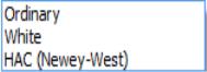
To specify the use of White heteroskedasticity robust standard errors, we will select in the dropdown menu on the tab. By default, EViews will estimate the using the method with as specified in
Equation (23.3).
Output from TSLS
Below we show the output from a regression of LOG(PACKPC) on a constant and LOG(RAVGPRS) and LOG(PERINC), with instrument list “LOG(PERINC) RTAXSO RTAXS”.
EViews identifies the estimation procedure, as well as the list of instruments in the header. This information is followed by the usual coefficient, t-statistics, and asymptotic p-values.
The summary statistics reported at the bottom of the table are computed using the formulae outlined in
“Summary Statistics”. Bear in mind that all reported statistics are only asymptotically valid. For a discussion of the finite sample properties of TSLS, see Johnston and DiNardo (1997, p. 355–358) or Davidson and MacKinnon (1993, p. 221–224).
Three other summary statistics are reported: “Instrument rank”, the “J-statistic” and the “Prob(J-statistic)”. The Instrument rank is simply the rank of the instrument matrix, and is equal to the number of instruments used in estimation. The J-statistic is calculated as:
 | (23.4) |
where

are the regression residuals. See
“Generalized Method of Moments” for additional discussion of the
J-statistic.
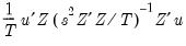
EViews uses the
structural residuals 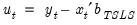
in calculating the summary statistics. For example, the default estimator of the standard error of the regression used in the covariance calculation is:
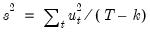 | (23.5) |
These structural, or regression, residuals should be distinguished from the
second stage residuals that you would obtain from the second stage regression if you actually computed the two-stage least squares estimates in two separate stages. The second stage residuals are given by
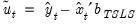
, where the

and

are the fitted values from the first-stage regressions.
We caution you that some of the reported statistics should be interpreted with care. For example, since different equation specifications will have different instrument lists, the reported

for TSLS can be negative even when there is a constant in the equation.
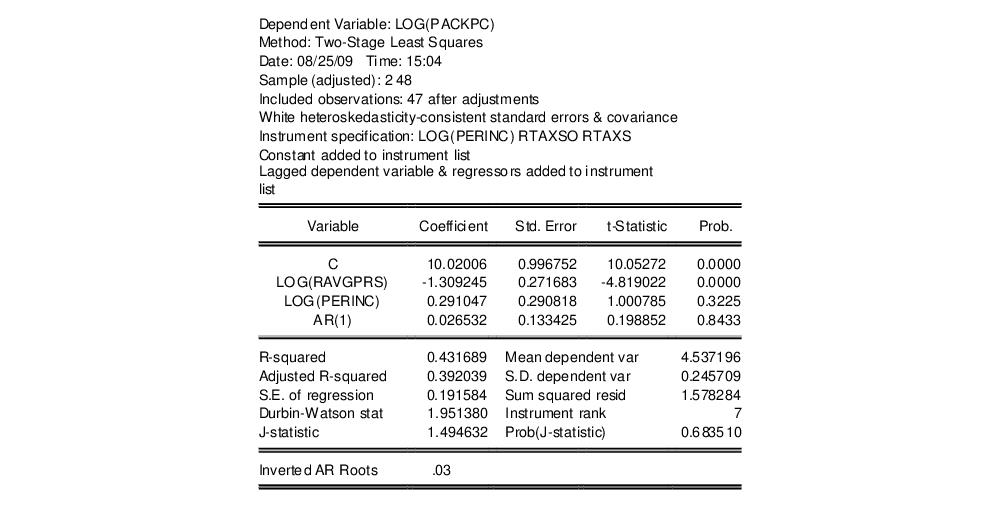
TSLS with AR errors
You can adjust your TSLS estimates to account for serial correlation by adding AR terms to your equation specification. EViews will automatically transform the model to a nonlinear least squares problem, and estimate the model using instrumental variables. Details of this procedure may be found in Fair (1984, p. 210–214). The output from TSLS with an AR(1) specification using the default settings with a tighter convergence tolerance looks as follows:
The Options button in the estimation box may be used to change the iteration limit and convergence criterion for the nonlinear instrumental variables procedure.
First-order AR errors
Suppose your specification is:
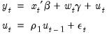 | (23.6) |
where

is a vector of endogenous variables, and

is a vector of predetermined variables, which, in this context, may include lags of the dependent variable

. is a vector of instrumental variables not in

that is large enough to identify the parameters of the model.
In this setting, there are important technical issues to be raised in connection with the choice of instruments. In a widely cited result, Fair (1970) shows that if the model is estimated using an iterative Cochrane-Orcutt procedure, all of the lagged left- and right-hand side variables
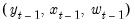
must be included in the instrument list to obtain consistent estimates. In this case, then the instrument list should include:
 | (23.7) |
EViews estimates the model as a nonlinear regression model so that Fair’s warning does not apply. Estimation of the model does, however, require specification of additional instruments to satisfy the instrument order condition for the transformed specification. By default, the first-stage instruments employed in TSLS are formed as if one were running Cochrane-Orcutt using Fair’s prescription. Thus, if you omit the lagged left- and right-hand side terms from the instrument list, EViews will, by default, automatically add the lagged terms as instruments. This addition will be noted in your output.
You may instead instruct EViews not to add the lagged left- and right-hand side terms as instruments. In this case, you are responsible for adding sufficient instruments to ensure the order condition is satisfied.
Higher Order AR errors
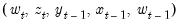
The AR(1) results extend naturally to specifications involving higher order serial correlation. For example, if you include a single AR(4) term in your model, the natural instrument list will be:
 | (23.8) |
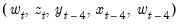
If you include AR terms from 1 through 4, one possible instrument list is:
 | (23.9) |
Note that while conceptually valid, this instrument list has a large number of overidentifying instruments, which may lead to computational difficulties and large finite sample biases (Fair (1984, p. 214), Davidson and MacKinnon (1993, p. 222-224)). In theory, adding instruments should always improve your estimates, but as a practical matter this may not be so in small samples.
In this case, you may wish to turn off the automatic lag instrument addition and handle the additional instrument specification directly.
Examples
Suppose that you wish to estimate the consumption function by two-stage least squares, allowing for first-order serial correlation. You may then use two-stage least squares with the variable list,
cons c gdp ar(1)
and instrument list:
c gov log(m1) time cons(-1) gdp(-1)
Notice that the lags of both the dependent and endogenous variables (CONS(–1) and GDP(–1)), are included in the instrument list.
Similarly, consider the consumption function:
cons c cons(-1) gdp ar(1)
A valid instrument list is given by:
c gov log(m1) time cons(-1) cons(-2) gdp(-1)
Here we treat the lagged left and right-hand side variables from the original specification as predetermined and add the lagged values to the instrument list.
Lastly, consider the specification:
cons c gdp ar(1 to 4)
Adding all of the relevant instruments in the list, we have:
c gov log(m1) time cons(-1) cons(-2) cons(-3) cons(-4) gdp(-1) gdp(-2) gdp(-3) gdp(-4)
TSLS with MA errors
You can also estimate two-stage least squares variable problems with MA error terms of various orders. To account for the presence of MA errors, simply add the appropriate terms to your specification prior to estimation.
Illustration
Suppose that you wish to estimate the consumption function by two-stage least squares, accounting for first-order moving average errors. You may then use two-stage least squares with the variable list,
cons c gdp ma(1)
and instrument list:
c gov log(m1) time
EViews will add both first and second lags of CONS and GDP to the instrument list.
Technical Details
Most of the technical details are identical to those outlined above for AR errors. EViews transforms the model that is nonlinear in parameters (employing backcasting, if appropriate) and then estimates the model using nonlinear instrumental variables techniques.
Recall that by default, EViews augments the instrument list by adding lagged dependent and regressor variables corresponding to the AR lags. Note however, that each MA term involves an infinite number of AR terms. Clearly, it is impossible to add an infinite number of lags to the instrument list, so that EViews performs an ad hoc approximation by adding a truncated set of instruments involving the MA order and an additional lag. If for example, you have an MA(5), EViews will add lagged instruments corresponding to lags 5 and 6.
Of course, you may instruct EViews not to add the extra instruments. In this case, you are responsible for adding enough instruments to ensure the instrument order condition is satisfied.