Generalized Method of Moments
We offer here a brief description of the Generalized Method of Moments (GMM) estimator, paying particular attention to issues of weighting matrix estimation and coefficient covariance calculation. Or treatment parallels the excellent discussion in Hayashi (2000). Those interested in additional detail are encouraged to consult one of the many comprehensive surveys of the subject.
The GMM Estimator
The starting point of GMM estimation is the assumption that there are a set of

moment conditions that the

-dimensional parameters of interest,

should satisfy. These moment conditions can be quite general, and often a particular model has more specified moment conditions than parameters to be estimated. Thus, the vector of

moment conditions may be written as:
 | (23.24) |
In EViews (as in most econometric applications), we restrict our attention to moment conditions that may be written as an orthogonality condition between the residuals of an equation,
, and a set of

instruments

:
 | (23.25) |
The traditional Method of Moments estimator is defined by replacing the moment conditions in
Equation (23.24) with their sample analog:
 | (23.26) |
and finding the parameter vector

which solves this set of

equations.
When there are more moment conditions than parameters (

), the system of equations given in
Equation (23.26) may not have an exact solution. Such as system is said to be
overidentified. Though we cannot generally find an exact solution for an overidentified system, we can reformulate the problem as one of choosing a

so that the sample moment

is as “close” to zero as possible, where “close” is defined using the quadratic form:
 | (23.27) |
as a measure of distance. The possibly random, symmetric and positive-definite

matrix

is termed the
weighting matrix since it acts to weight the various moment conditions in constructing the distance measure. The
Generalized Method of Moments estimate is defined as the

that minimizes
Equation (23.27).
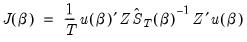
As with other instrumental variable estimators, for the GMM estimator to be identified, there must be at least as many instruments as there are parameters in the model. In models where there are the same number of instruments as parameters, the value of the optimized objective function is zero. If there are more instruments than parameters, the value of the optimized objective function will be greater than zero. In fact, the value of the objective function, termed the J-statistic, can be used as a test of over-identifying moment conditions.
Under suitable regularity conditions, the GMM estimator is consistent and

asymptotically normally distributed,
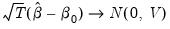 | (23.28) |
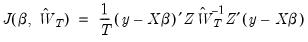
The asymptotic covariance matrix

of

is given by
 | (23.29) |
for
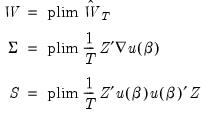 | (23.30) |
where

is both the asymptotic variance of

and the long-run covariance matrix of the vector process

.
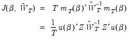
In the leading case where the

are the residuals from a linear specification so that
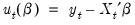
, the GMM objective function is given by
 | (23.31) |
and the GMM estimator yields the unique solution
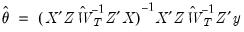
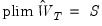
. The asymptotic covariance matrix is given by
Equation (23.27), with
 | (23.32) |
It can be seen from this formation that both two-stage least squares and ordinary least squares estimation are both special cases of GMM estimation. The two-stage least squares objective is simply the GMM objective function multiplied by

using weighting matrix
. Ordinary least squares is equivalent to two-stage least squares objective with the instruments set equal to the derivatives of

, which in the linear case are the regressors.
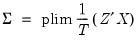
Choice of Weighting Matrix
An important aspect of specifying a GMM estimator is the choice of the weighting matrix,

. While any sequence of symmetric positive definite weighting matrices

will yield a consistent estimate of

,
Equation (23.29) implies that the choice of

affects the asymptotic variance of the GMM estimator. Hansen (1992) shows that an
asymptotically efficient, or
optimal GMM estimator of

may be obtained by choosing

so that it converges to the inverse of the long-run covariance matrix

:
 | (23.33) |
Intuitively, this result follows since we naturally want to assign less weight to the moment conditions that are measured imprecisely. For a GMM estimator with an optimal weighting matrix, the asymptotic covariance matrix of

is given by
 | (23.34) |
Implementation of optimal GMM estimation requires that we obtain estimates of

. EViews offers four basic methods for specifying a weighting matrix:
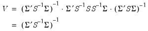
• : the two-stage least squares weighting matrix is given by
where

is an estimator of the residual variance based on an initial estimate of

. The estimator for the variance will be

or the no d.f. corrected equivalent, depending on your settings for the coefficient covariance calculation.
• : the White weighting matrix is a heteroskedasticity consistent estimator of the long-run covariance matrix of

based on an initial estimate of

.
• : the HAC weighting matrix is a heteroskedasticity and autocorrelation consistent estimator of the long-run covariance matrix of

based on an initial estimate of

.
• : this method allows you to provide your own weighting matrix (specified as a sym matrix containing a scaled estimate of the long-run covariance

).
For related discussion of the and robust standard error estimators, see
“Robust Standard Errors”.
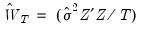
Weighting Matrix Iteration
As noted above, both the White and HAC weighting matrix estimators require an initial consistent estimate of

. (Technically, the two-stage least squares weighting matrix also requires an initial estimate of

, though these values are irrelevant since the resulting

does not affect the resulting estimates).
Accordingly, computation of the optimal GMM estimator with White or HAC weights often employs a variant of the following procedure:
1. Calculate initial parameter estimates

using TSLS
2. Use the

estimates to form residuals

3. Form an estimate of the long-run covariance matrix of

,

, and use it to compute the optimal weighting matrix

4. Minimize the GMM objective function with weighting matrix

 | (23.35) |
with respect to

to form updated parameter estimates.
We may generalize this procedure by repeating steps 2 through 4 using

as our initial parameter estimates, producing updated estimates

. This iteration of weighting matrix and coefficient estimation may be performed a fixed number of times, or until the coefficients converge so that

to a sufficient degree of precision.
An alternative approach due to Hansen, Heaton and Yaron (1996) notes that since the optimal weighting matrix is dependent on the parameters, we may rewrite the GMM objective function as
 | (23.36) |
where the weighting matrix is a direct function of the

being estimated. The estimator which minimizes
Equation (23.36) with respect to

has been termed the
Continuously Updated Estimator (CUE).
Linear Equation Weight Updating
For equations that are linear in their coefficients, EViews offers three weighting matrix updating options: the , the , and the method.
As the names suggests, the method repeats steps 2-5 above

times, while the repeats the steps until the parameter estimates converge. The approach is based on
Equation (23.36).
Somewhat confusingly, the with a single weight step is sometimes referred to in the literature as the 2-step GMM estimator, the first step being defined as the initial TSLS estimation. EViews views this as a 1-step estimator since there is only a single optimal weight matrix computation.
Non-linear Equation Weight Updating
For equations that are non-linear in their coefficients, EViews offers five different updating algorithms: , , , , and . The methods for non-linear specifications are generally similar to their linear counterparts, with differences centering around the fact that the parameter estimates for a given weighting matrix in step 4 must now be calculated using a non-linear optimizer, which itself involves iteration.
All of the non-linear weighting matrix update methods begin with

obtained from two-stage least squares estimation in which the coefficients have been iterated to convergence.
The procedure is analogous to the linear procedure outlined above, but with the non-linear optimization for the parameters in each step 4 iterated to convergence. Similarly, the method follows the same approach as the method, with full non-linear optimization of the parameters in each step 4.
The method differs from in that only a single iteration of the non-linear optimizer, rather than iteration to convergence, is conducted in step 4. The iterations are therefore simultaneous in the sense that each weight iteration is paired with a coefficient iteration.
performs a single weight iteration after the initial two-stage least squares estimates, and then a single iteration of the non-linear optimizer based on the updated weight matrix.
The approach is again based on
Equation (23.36).
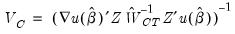
Coefficient Covariance Calculation
Having estimated the coefficients of the model, all that is left is to specify a method of computing the coefficient covariance matrix. We will consider two basic approaches, one based on a family of estimators of the asymptotic covariance given in
Equation (23.29), and a second, due to Windmeijer (2000, 2005), which employs a bias-corrected estimator which take into account the variation of the initial parameter estimates.
Conventional Estimators
Using
Equation (23.29) and inserting estimators and sample moments, we obtain an estimator for the asymptotic covariance matrix of

:
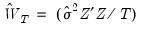
 | (23.37) |
where
 | (23.38) |
Notice that the estimator depends on both the final coefficient estimates

and the

used to form the estimation weighting matrix, as well as an additional estimate of the long-run covariance matrix

. For weight update methods which iterate the weights until the coefficients converge the two sets of coefficients will be identical.
EViews offers a number of different covariance specifications of this form, , , , , , , , and , each corresponding to a different estimator for

.
Of these, and are the most commonly employed coefficient covariance methods. Both methods compute

using the estimation weighting matrix specification (
i.e. if was chosen as the estimation weighting matrix, then will also be used for estimating

).
• uses the previously computed estimate of the long-run covariance matrix to form
. The asymptotic covariance matrix simplifies considerably in this case so that
.
• performs one more step 3 in the iterative estimation procedure, computing an estimate of the long-run covariance using the final coefficient estimates to obtain
. Since this method relies on the iterative estimation procedure, it is not available for equations estimated by CUE.
In cases, where the weighting matrices are iterated to convergence, these two approaches will yield identical results.
The remaining specifications compute estimates of

at the final parameters

using the indicated long-run covariance method. You may use these methods to estimate your equation using one set of assumptions for the weighting matrix
, while you compute the coefficient covariance using a different set of assumptions for

.
The primary application for this mixed weighting approach is in computing robust standard errors. Suppose, for example, that you want to estimate your equation using TSLS weights, but with robust standard errors. Selecting for the estimation weighting matrix and for the covariance calculation method will instruct EViews to compute TSLS estimates with White coefficient covariances and standard errors. Similarly, estimating with estimation weights and covariance weights produces TSLS estimates with HAC coefficient covariances and standard errors.
Note that it is possible to choose combinations of estimation and covariance weights that, while reasonable, are not typically employed. You may, for example, elect to use White estimation weights with HAC covariance weights, or perhaps HAC estimation weights using one set of HAC options and HAC covariance weights with a different set of options. It is also possible, though not recommended, to construct odder pairings such as HAC estimation weights with TSLS covariance weights.
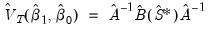
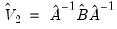
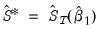
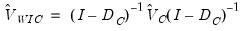
Windmeijer Estimator
Various Monte Carlo studies (e.g. Arellano and Bond 1991) have shown that the above covariance estimators can produce standard errors that are downward biased in small samples. Windmeijer (2000, 2005) observes that part of this downward bias is due to extra variation caused by the initial weight matrix estimation being itself based on consistent estimates of the equation parameters.
Following this insight it is possible to calculate bias-corrected standard error estimates which take into account the variation of the initial parameter estimates. Windmeijer provides two forms of bias corrected standard errors; one for GMM models estimated in a one-step (one optimal GMM weighting matrix) procedure, and one for GMM models estimated using an iterate-to-convergence procedure.
The Windmeijer corrected variance-covariance matrix of the one-step estimator is given by:
 | (23.39) |
where:

, the estimation default covariance estimator
, the updated weighting matrix (at final parameter estimates)
, the estimation updated covariance estimator where
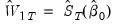
, the estimation weighting matrix (at initial parameter estimates)
, the initial weighting matrix

is a matrix whose

th column is given by

:
The Windmeijer iterate-to-convergence variance-covariance matrix is given by:
 | (23.40) |
where:
, the estimation default covariance estimator

, the GMM weighting matrix at converged parameter estimates
Weighted GMM
Weights may also be used in GMM estimation. The objective function for weighted GMM is,
 | (23.41) |
where

is the long-run covariance of

where we now use

to indicate the diagonal matrix with observation weights

.
The default reported standard errors are based on the covariance matrix estimate given by:
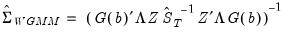 | (23.42) |
where

.
Estimation by GMM in EViews
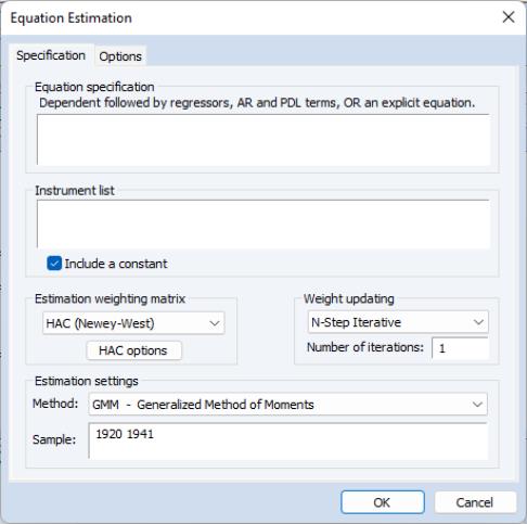
To estimate an equation by GMM, either create a new equation object by selecting , or press the button in the toolbar of an existing equation. From the dialog choose Estimation Method: GMM. The estimation specification dialog will change as depicted below.
To obtain GMM estimates in EViews, you need to write the moment condition as an orthogonality condition between an expression including the parameters and a set of instrumental variables. There are two ways you can write the orthogonality condition: with and without a dependent variable.
If you specify the equation either by listing variable names or by an expression with an equal sign, EViews will interpret the moment condition as an orthogonality condition between the instruments and the residuals defined by the equation. If you specify the equation by an expression without an equal sign, EViews will orthogonalize that expression to the set of instruments.
You must also list the names of the instruments in the Instrument list edit box. For the GMM estimator to be identified, there must be at least as many instrumental variables as there are parameters to estimate. EViews will, by default, add a constant to the instrument list. If you do not wish a constant to be added to the instrument list, the check box should be unchecked.
For example, if you type,
Equation spec: y c x
Instrument list: c z w
the orthogonality conditions are given by:
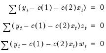 | (23.43) |
If you enter the specification,
Equation spec: c(1)*log(y)+x^c(2)
Instrument list: c z z(-1)
the orthogonality conditions are:
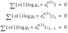 | (23.44) |
Beneath the box there are two dropdown menus that let you set the and the .
The dropdown specifies the type of GMM weighting matrix that will be used during estimation. You can choose from , , , and . If you select then a button appears that lets you set the weighting matrix computation options. If you select , you will be prompted for a cluster series. If you select you must enter the name of a symmetric matrix in the workfile containing an estimate of the weighting matrix (long-run covariance) scaled by the number of observations

). Note that the matrix must have as many columns as the number of instruments specified.
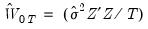
The

matrix can be retrieved from any equation estimated by GMM using the
@instwgt data member (see
“Equation Data Members”).
@instwgt returns

which is an implicit estimator of the long-run covariance scaled by the number of observations.
For example, for GMM equations estimated using the weighting matrix, will contain

(where the estimator for the variance will use

or the no d.f. corrected equivalent, depending on your options for coefficient covariance calculation). Equations estimated with a weighting matrix will return

.
Storing the user weighting matrix from one equation, and using it during the estimation of a second equation may prove useful when computing diagnostics that involve comparing J-statistics between two different equations.
The dropdown menu lets you set the estimation algorithm type. For linear equations, you can choose between , , and . For non-linear equations, the choice is between , , , and .
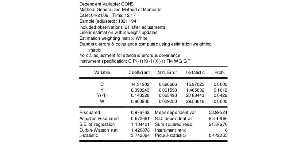
To illustrate estimation of GMM models in EViews, we estimate the same Klein model introduced in
“Estimating LIML and K-Class in EViews”, as again replicated by Greene 2008 (p. 385). We again estimate the Consumption equation, where consumption (CONS) is regressed on a constant, private profits (Y), lagged private profits (Y(-1)), and wages (W) using data in “Klein.WF1”. The instruments are a constant, lagged corporate profits (P(-1)), lagged capital stock (K(-1)), lagged GNP (X(-1)), a time trend (TM), Government wages (WG), Government spending (G) and taxes (T). Greene uses the weighting matrix, and an updating procedure, with set to 2. The results of this estimation are shown below:
The EViews output header shows a summary of the estimation type and settings, along with the instrument specification. Note that in this case the header shows that the equation was linear, with a 2 step iterative weighting update performed. It also shows that the weighing matrix type was White, and this weighting matrix was used for the covariance matrix, with no degree of freedom adjustment.
Following the header the standard coefficient estimates, standard errors, t-statistics and associated p-values are shown. Below that information are displayed the summary statistics. Apart from the standard statistics shown in an equation, the instrument rank (the number of linearly independent instruments used in estimation) is also shown (8 in this case), and the J-statistic and associated p-value is also shown.
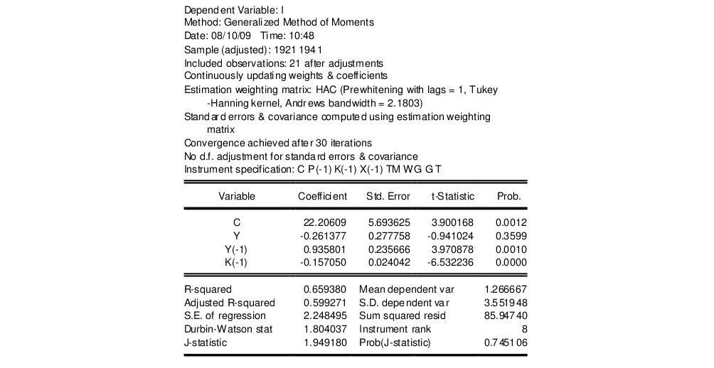
As a second example, we also estimate the equation for Investment. Investment (I) is regressed on a constant, private profits (Y), lagged private profits (Y(-1)) and lagged capital stock (K-1)). The instruments are again a constant, lagged corporate profits (P(-1)), lagged capital stock (K(-1)), lagged GNP (X(-1)), a time trend (TM), Government wages (WG), Government spending (G) and taxes (T).
Unlike Greene, we will use a weighting matrix, with pre-whitening (fixed at 1 lag), a Tukey-Hanning kernel with Andrews Automatic Bandwidth selection. We will also use the weighting updating procedure. The output from this equation is show below:
Note that the header information for this equation shows slightly different information from the previous estimation. The inclusion of the weighting matrix yields information on the prewhitening choice (lags = 1), and on the kernel specification, including the bandwidth that was chosen by the Andrews procedure (2.1803). Since the procedure is used, the number of optimization iterations that took place is reported (39).