Technical Discussion
Our basic discussion and notation follows the framework of Andrews (1991) and Hansen (1992a).
Consider a sequence of mean-zero random

-vectors

that may depend on a

‑vector of parameters

, and let

where

is the true value of

. We are interested in estimating the LRCOV matrix

,
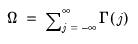 | (60.32) |
where
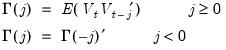 | (60.33) |
is the autocovariance matrix of

at lag

. When

is second-order stationary,

equals

times the spectral density matrix of

evaluated at frequency zero (Hansen 1982, Andrews 1991, Hamilton 1994).
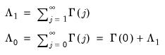
Closely related to

are two measures of the
one-sided LRCOV matrix:
 | (60.34) |
The matrix

, which we term the
strict one-sided LRCOV, is the sum of the lag covariances, while the

also includes the contemporaneous covariance

. The two-sided LRCOV matrix

is related to the one-sided matrices through
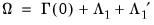
and
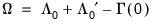
.
Despite the important role the one-sided LRCOV matrix plays in the literature, we will focus our attention on

, since results are generally applicable to all three measures; exception will be made for specific issues that require additional comment.
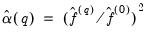
In the econometric literature, methods for using a consistent estimator

and the corresponding

to form a consistent estimate of

are often referred to as
heteroskedasticity and autocorrelation consistent (HAC) covariance matrix estimators.
There have been three primary approaches to estimating

:
1. The
nonparametric kernel approach (Andrews 1991, Newey-West 1987) forms estimates of

by taking a weighted sum of the sample autocovariances of the observed data.
2. The
parametric VARHAC approach (Den Haan and Levin 1997) specifies and fits a parametric time series model to the data, then uses the estimated model to obtain the implied autocovariances and corresponding

.
3. The
prewhitened kernel approach (Andrews and Monahan 1992) is a hybrid method that combines the first two approaches, using a parametric model to obtain residuals that “whiten” the data, and a nonparametric kernel estimator to obtain an estimate of the LRCOV of the whitened data. The estimate of

is obtained by “recoloring” the prewhitened LRCOV to undo the effects of the whitening transformation.
Below, we offer a brief description of each of these approaches, paying particular attention to issues of kernel choice, bandwidth selection, and lag selection.
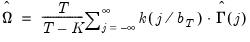
Nonparametric Kernel
The class of kernel HAC covariance matrix estimators in Andrews (1991) may be written as:
 | (60.35) |
where the sample autocovariances

are given by
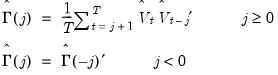 | (60.36) |

is a symmetric kernel (or lag window) function that, among other conditions, is continous at the origin and satisfies

for all

with

, and

is a bandwidth parameter. The leading

term is an
optional correction for degrees-of-freedom associated with the estimation of the

parameters in

.
The choice of a kernel function and a value for the bandwidth parameter completely characterizes the kernel HAC estimator.
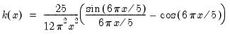
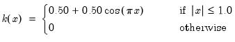
Kernel Functions
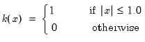
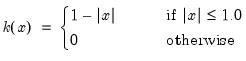
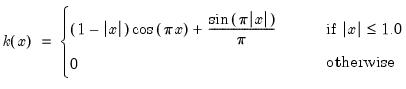
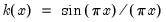
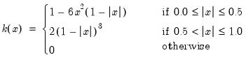
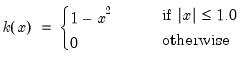
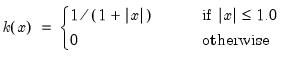
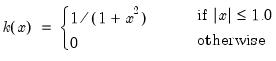
There are a large number of kernel functions that satisfy the required conditions. EViews supports use of the following kernel shapes:
Note that

for

for all kernels with the exception of the Daniell and the Quadratic Spectral. The Daniell kernel is presented in truncated form in Neave (1972), but EViews uses the more common untruncated form. The Bartlett kernel is sometimes referred to as the Fejer kernel (Neave 1972).
A wide range of kernels have been employed in HAC estimation. The truncated uniform is used by Hansen (1982) and White (1984), the Bartlett kernel is used by Newey and West (1987), and the Parzen is used by Gallant (1987). The Tukey-Hanning and Quadratic Spectral were introduced to the econometrics literature by Andrews (1991), who shows that the latter is optimal in the sense of minimizing the asymptotic truncated MSE of the estimator (within a particular class of kernels). The remaining kernels are discussed in Parzen (1958, 1961, 1967).
Bandwidth
The bandwidth

operates in concert with the kernel function to determine the weights for the various sample autocovariances in
Equation (60.35). While some authors restrict the bandwidth values to integers, we follow Andrews (1991) who argues in favor of allowing real valued bandwidths.
To construct an operational nonparametric kernel estimator, we must choose a value for the bandwidth

. Under general conditions (Andrews 1991), consistency of the kernel estimator requires that

is chosen so that

and

as

. Alternately, Kiefer and Vogelsang (2002) propose setting

in a testing context.
For the great majority of supported kernels
for

so that the bandwidth acts indirectly as a lag truncation parameter. Relating

to the corresponding integer lag number of included lags

requires, however, examining the properties of the kernel at the endpoints
. For kernel functions where

(
e.g., Truncated, Parzen-Geometric, Tukey-Hanning),

is simply a real-valued truncation lag, with at most
autocovariances having non-zero weight. Alternately, for kernel functions where

(
e.g., Bartlett, Bohman, Parzen), the relationship is slightly more complex, with
autocovariances entering the estimator with non-zero weights.
The varying relationship between the bandwidth and the lag-truncation parameter implies that one should examine the kernel function when choosing bandwidth values to match computations that are quoted in lag truncation form. For example, matching Newey-West’s (1987) Bartlett kernel estimator which uses

weighted autocovariance lags requires setting

. In contrast, Hansen’s (1982) or White’s (1984) estimators, which sum the first

unweighted autocovariances, should be implemented using the Truncated kernel with

.
Automatic Bandwidth Selection
Theoretical results on the relationship between bandwidths and the asymptotic truncated MSE of the kernel estimator provide finer discrimination in the rates at which bandwidths should increase. The optimal bandwidths may be written in the form:
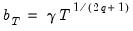 | (60.37) |
where

is a constant, and

is a parameter that depends on the kernel function that you select (Parzen 1958, Andrews 1991). For the Bartlett and Parzen-Geometric kernels


should grow (at most) at the rate

. The Truncated kernel does not have an theoretical optimal rate, but Andrews (1991) reports Monte Carlo simulations that suggest that

works well. The remaining EViews supported kernels have

so their optimal bandwidths grow at rate

(though we point out that Daniell kernel does not satisfy the conditions for the optimal bandwidth theorems).
While theoretically useful, knowledge of the rate at which bandwidths should increase as

does not tell us the optimal bandwidth for a given sample size, since the constant

remains unspecified.
Andrews (1991) and Newey and West (1994) offer two approaches to estimating

. We may term these techniques
automatic bandwidth selection methods, since they involve estimating the optimal bandwidth from the data, rather than specifying a value
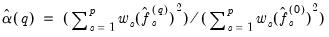
a priori. Both the Andrews and Newey-West estimators for

may be written as:
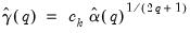 | (60.38) |
where

and the constant

depend on properties of the selected kernel and

is an estimator of

, a measure of the smoothness of the spectral density at frequency zero that depends on the autocovariances

. Substituting into
Equation (60.37), the resulting plug-in estimator for the optimal automatic bandwidth is given by:
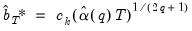 | (60.39) |
The

that one uses depends on properties of the selected kernel function. The Bartlett and Parzen-Geometric kernels should use

since they have

.

should be used for the other EViews supported kernels which have

. The Truncated kernel does not have a theoretically proscribed choice, but Andrews recommends using

. The Daniell kernel has

, though we remind you that it does not satisfy the conditions for Andrews’s theorems.
“Kernel Function Properties” summarizes the values of

and

for the various kernel functions.
It is of note that the Andrews and Newey-West estimators both require an estimate of

that requires forming preliminary estimates of

and the smoothness of

. Andrews and Newey-West offer alternative methods for forming these estimates.
Andrews Automatic Selection
The Andrews (1991) method estimates

parametrically: fitting a simple parametric time series model to the original data, then deriving the autocovariances

and corresponding

implied by the estimated model.
Andrews derives

formulae for several parametric models, noting that the choice between specifications depends on a tradeoff between simplicity and parsimony on one hand and flexibility on the other. EViews employs the parsimonius approach used by Andrews in his Monte Carlo simulations, estimating

-univariate AR(1) models (one for each element of

), then combining the estimated coefficients into an estimator for

.
For the univariate AR(1) approach, we have:
 | (60.40) |
where

are parametric estimators of the smoothness of the spectral density for the

-th variable (Parzen’s (1957)

‑th generalized spectral derivatives) at frequency zero. Estimators for

are given by:
 | (60.41) |
for

and

, where

are the estimated autocovariances at lag

implied by the univariate AR(1) specification for the

‑th variable.
Substituting the univariate AR(1) estimated coefficients

and standard errors

into the theoretical expressions for

, we have:
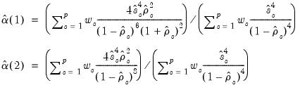 | (60.42) |
which may be inserted into
Equation (60.39) to obtain expressions for the optimal bandwidths.
Lastly, we note that the expressions for

depend on the weighting vector

which governs how we combine the individual

into a single measure of relative smoothness. Andrews suggests using either

for all

or

for all but the instrument corresponding to the intercept in regression settings. EViews adopts the first suggestion, setting

for all

.
Newey-West Automatic Selection
Newey-West (1994) employ a nonparametric approach to estimating

. In contrast to Andrews who computes parametric estimates of the individual

, Newey-West uses a Truncated kernel estimator to estimate the

corresponding to aggregated data.
First, Newey and West define, for various lags, the scalar autocovariance estimators:
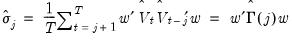 | (60.43) |
The

may either be viewed as the sample autocovariance of a weighted linear combination of the data using weights

, or as a weighted combination of the sample autocovariances.
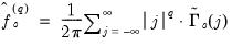
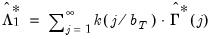
Next, Newey and West use the

to compute nonparametric truncated kernel estimators of the Parzen measures of smoothness:
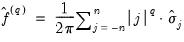 | (60.44) |
for

. These nonparametric estimators are weighted sums of the scalar autocovariances

obtained above for

from

to

, where

, which Newey and West term the
lag selection parameter, may be viewed as the bandwidth of a kernel estimator for

.
The Newey and West estimator for

may then be written as:
 | (60.45) |
for

. This expression may be inserted into
Equation (60.39) to obtain the expression for the plug-in optimal bandwidth estimator.
In comparing the Andrews estimator
Equation (60.42) with the Newey-West estimator
Equation (60.45) we see two very different methods of distilling results from the

-dimensions of the original data into a scalar measure

. Andrews computes parametric estimates of the generalized derivatives for the

individual elements, then aggregates the estimates into a single measure. In contrast, Newey and West aggregate early, forming linear combinations of the autocovariance matrices, then use the scalar results to compute nonparametric estimators of the Parzen smoothness measures.
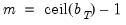
To implement the Newey-West optimal bandwidth selection method we require a value for

, the lag-selection parameter, which governs how many autocovariances to use in forming the nonparametric estimates of

. Newey and West show that

should increase at (less than) a rate that depends on the properties of the kernel. For the Bartlett and the Parzen-Geometric kernels, the rate is

. For the Quadratic Spectral kernel, the rate is

. For the remaining kernels, the rate is

(with the exception of the Truncated and the Daniell kernels, for which the Newey-West theorems do not apply).
In addition, one must choose a weight vector

. Newey-West (1987) leave open the choice of

, but follow Andrew’s (1991) suggestion of

for all but the intercept in their Monte Carlo simulations. EViews differs from this choice slightly, setting

for all

.
Parametric VARHAC
Den Haan and Levin (1997) advocate the use of parametric methods, notably VARs, for LRCOV estimation. The VAR spectral density estimator, which they term
VARHAC, involves estimating a parametric VAR model to filter the

, computing the contemporaneous covariance of the filtered data, then using the estimates from the VAR model to obtain the implied autocovariances and corresponding LRCOV matrix of the original data.
Suppose we fit a VAR(

) model to the

. Let

be the

matrix of estimated

-th order AR coefficients,

. Then we may define the innovation (filtered) data and estimated innovation covariance matrix as:
 | (60.46) |
and
 | (60.47) |
Given an estimate of the innovation contemporaneous variance matrix

and the VAR coefficients

, we can compute the implied theoretical autocovariances

of

. Summing the autocovariances yields a parametric estimator for

, given by:
 | (60.48) |
where
 | (60.49) |
Implementing VARHAC requires a specification for

, the order of the VAR. Den Haan and Levin use model selection criteria (AIC or BIC-Schwarz) using a maximum lag of

to determine the lag order, and provide simulations of the performance of estimator using data-dependent lag order.
The corresponding VARHAC estimators for the one-sided matrices

and

do not have simple expressions in terms of

and

. We can, however, obtain insight into the construction of the one-sided VARHAC LRCOVs by examining results for the VAR(1) case. Given estimation of a VAR(1) specification, the estimators for the one-sided long-run variances may be written as:
 | (60.50) |
Both estimators require estimates of the VAR(1) coefficient estimates

, as well as an estimate of

, the contemporaneous covariance matrix of

.
One could, as in Park and Ogaki (1991) and Hansen (1992b), use the sample covariance matrix
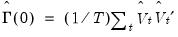
so that the estimates of

and

employ a mix of parametric and non-parametric autocovariance estimates. Alternately, in keeping with the spirit of the parametric methodology, EViews constructs a parametric estimator

using the estimated VAR(1) coefficients

and

.
Prewhitened Kernel
Andrews and Monahan (1992) propose a simple modification of the kernel estimator which performs a parametric VAR prewhitening step to reduce autocorrelation in the data followed by kernel estimation performed on the whitened data. The resulting prewhitened LRVAR estimate is then recolored to undo the effects of the transformation. The Andrews and Monahan approach is a hybrid that combines the parametric VARHAC and nonparametric kernel techniques.
There is evidence (Andrews and Monahan 1992, Newey-West 1994) that this prewhitening approach has desirable properties, reducing bias, improving confidence interval coverage probabilities and improving sizes of test statistics constructed using the kernel HAC estimators.
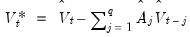
The Andrews and Monahan estimator follows directly from our earlier discussion. As in a VARHAC, we first fit a VAR(

) model to the

and obtain the whitened data (residuals):
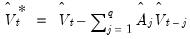 | (60.51) |
In contrast to the VAR specification in the VARHAC estimator, the prewhitening VAR specification is not necessarily believed to be the true time series model, but is merely a tool for obtaining

values that are closer to white-noise. (In addition, Andrews and Monahan adjust their VAR(1) estimates to avoid singularity when the VAR is near unstable, but EViews does not perform this eigenvalue adjustment.)
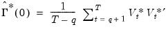
Next, we obtain an estimate of the LRCOV of the whitened data by applying a kernel estimator to the residuals:
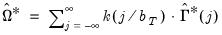 | (60.52) |
where the sample autocovariances

are given by
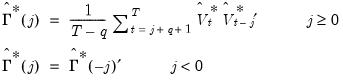 | (60.53) |
Lastly, we recolor the estimator to obtain the VAR prewhitened kernel LRCOV estimator:
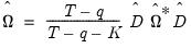 | (60.54) |
The prewhitened kernel procedure differs from VARHAC only in the computation of the LRCOV of the residuals. The VARHAC estimator in
Equation (60.48) assumes that the residuals

are white noise so that the LRCOV may be estimated using the contemporaneous variance matrix

, while the prewhitening kernel estimator in
Equation (60.52) allows for residual heteroskedasticity and serial dependence through its use of the HAC estimator

. Accordingly, it may be useful to view the VARHAC procedure as a special case of the prewhitened kernel with

and

for

.
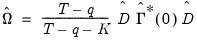
The recoloring step for one-sided prewhitened kernel estimators is complicated when we allow for HAC estimation of

(Park and Ogaki, 1991). As in the VARHAC setting, the expressions for one-sided LRCOVs are quite involved but the VAR(1) specification may be used to provide insight. Suppose that the VARHAC estimators of the one-sided LRCOV matrices defined in
Equation (60.50) are given by

and

, and let

be the
strict one-sided kernel estimator computed using the prewhitened data:
 | (60.55) |
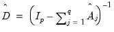
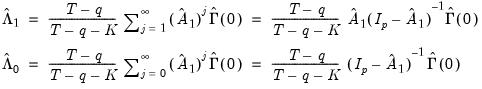
Then the prewhitened kernel one-sided LRCOV estimators are given by:
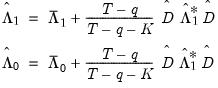 | (60.56) |