Solving the Model
Once the model specification is complete, you can solve the model. EViews can perform both deterministic and stochastic simulations.
A deterministic simulation consists of the following steps:
• The block structure of the model is analyzed.
• The variables in the model are bound to series in the workfile, according to the override settings and name aliasing rules of the scenario that is being solved. If an endogenous variable is being tracked and a series does not already exist in the workfile, a new series will be created. If an endogenous variable is not being tracked, a temporary series will be created to hold the results.
• The equations of the model are solved for each observation in the solution sample, using an iterative algorithm to compute values for the endogenous variables.
• Any temporary series which were created are deleted.
• The results are rounded to their final values.
A stochastic simulation follows a similar sequence, with the following differences:
• When binding the variables, a temporary series is created for every endogenous variable in the model. Additional series in the workfile are used to hold the statistics for the tracked endogenous variables. If bounds are being calculated, extra memory is allocated as working space for intermediate results.
• The model is solved repeatedly for different draws of the stochastic components of the model. If coefficient uncertainty is included in the model, then a new set of coefficients is drawn before each repetition (note that coefficient uncertainty is ignored in nonlinear equations, or linear equations specified with PDL terms). During the repetition, errors are generated for each observation in accordance with the residual uncertainty and the exogenous variable uncertainty in the model. At the end of each repetition, the statistics for the tracked endogenous variables are updated to reflect the additional results.
• If a comparison is being performed with an alternate scenario, then the same set of random residuals and exogenous variable shocks are applied to both scenarios during each repetition. This is done so that the deviation between the two is based only on differences in the exogenous and excluded variables, not on differences in random errors.
One source of models in which future values of endogenous variables may appear in equations are models of economic behavior in which expectations of future periods influence the decisions made in the current period. For example, when negotiating long term wage contracts, employers and employees must consider expected changes in prices over the duration of the contract. Similarly, when choosing to hold a security denominated in foreign currency, an individual must consider how the exchange rate is expected to change over the time that they hold the security.
Although the way that individuals form expectations is obviously complex, if the model being considered accurately captures the structure of the problem, we might expect the expectations of individuals to be broadly consistent with the outcomes predicted by the model. In the absence of any other information, we may choose to make this relationship hold exactly. Expectations of this form are often referred to as model consistent expectations.
Models Containing MA Terms
Solving models with equations that contain MA terms requires that we first obtain fitted values for the equation innovations in the pre-forecast sample period. For example, to perform dynamic forecasting of the values of

, beginning in period

using a simple MA(

):
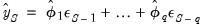 | (52.6) |
you require values for the pre-forecast sample innovations,
. Similarly, constructing a static forecast for a given period will require estimates of the

lagged innovations at every period in the forecast sample.
Initialization Methods
If your equation was estimated with backcasting turned on, EViews will, by default, perform backcasting to obtain initial values for model solution. If your equation is estimated with backcasting turned off, or if the forecast sample precedes the estimation sample, the initial values will be set to zero.
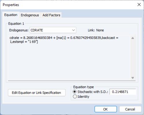
You may examine the equation specification in the model to determine whether backcasting was employed in estimation. The specification will include either the expression “BACKCAST=”, or “INITMA=” followed by an observation identifier for the first period of the estimation sample. As one might guess, “BACKCAST=” is used to indicate the use of backcasting in estimation; alternately, “INITMA=” indicates that the pre-sample values were initialized with zeros.
If neither “BACKCAST=” nor “INITMA=” is specified, the model will error when solved since EViews will be unable to obtain initial values for the forecast.
Here we see that the MA(1) equation for CDRATE in our model was estimated using “1 69” as the backcast estimation sample.
Backcast Methods
EViews offers alternate approaches for obtaining backcast estimates of the innovations when “BACKCAST=” is specified.
The estimation period method uses data for the estimation sample to compute backcast estimates. The post-backcast sample innovations are initialized to zero and backward recursion is employed to obtain estimates of the pre-estimation sample innovations. A forward recursion is then run to the end of the estimation sample and the resulting values are used as estimates of the innovations.
The alternative forecast available method offers different approaches for dynamic and static forecasting:
• For dynamic forecasting, EViews applies the backcasting procedure using data from the beginning of the estimation sample to either the beginning of the forecast period, or the end of the estimation sample, whichever comes first.
• For static forecasting, the backcasting procedure uses data from the beginning of the estimation sample to the end of the forecast period.
As before, the post-backcast sample innovations are set to zero and backward recursion is used to obtain estimates of the pre-estimation sample innovations, and forward recursion is used to obtain innovation estimates. Note that the forecast available method does not guarantee that the pre-sample forecast innovations match those employed in estimation.
See
“Forecasting with MA Errors” for additional discussion.
The backcast initialization method employed by EViews for an equation in model solution depends on a variety of factors:
• For equations estimated using EViews 6 and later, the initialization method is determined from the equation specification. If the equation was estimated using estimation sample backcasting, its specification will contain “BACKCAST=” and “ESTSMPL=” statements instructing EViews to backcast using the specified sample.
The example dialog above shows an equation estimated using the estimation sample backcasting method.
• For equations estimated prior to EViews 6, the model will only contain the “BACKCAST=” statement so that by default, the equation will be initialized using forecast available.
• In both cases, you may override the default settings by changing the specification of the equation in the model. To ensure that the equation backcasts using the forecast available method, simply delete the “ESTSMPL=” portion of the equation specification. To force the estimation sample method for model solution, you may add an “ESTSMPL=” statement to the equation specification.
Note that models containing post-EViews 6 equations solved in previous versions of EViews will always backcast using the forecast available method.
Models Containing Future Values
So far, we have assumed that the structure of the model allows us to solve each period of the model in sequence. This will not be true in the case where the equations of the model contain future (as well as past) values of the endogenous variables.
Consider a model where the equations have the form:
 | (52.7) |
where

is the complete set of equations of the model,

is a vector of all the endogenous variables,

is a vector of all the exogenous variables, and the parentheses follow the usual EViews syntax to indicate leads and lags.
Since solving the model for any particular period requires both past and future values of the endogenous variables, it is not possible to solve the model recursively in one pass. Instead, the equations from all the periods across which the model will be solved must be treated as a simultaneous system, and we will require terminal as well as initial conditions. For example, in the case with a single lead and a single lag and a sample that runs from

to

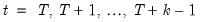
, we must effectively solve the entire stacked system:
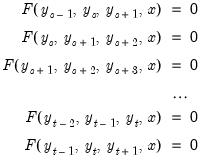 | (52.8) |
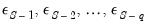
where the unknowns are

,

, ...,

the initial conditions are given by

and the terminal conditions are used to determine

. Note that if the leads or lags extend more than one period, we will require multiple periods of initial or terminal conditions.
EViews provides three methods for solving models such as these: Gauss-Seidel, E-Newton, and E-QNewton. All three are iterative procedures that attempt to reduce the change in the endogenous variables,

,

, ...,

, to zero as the model's equations are solved repeatedly. The first algorithm, Gauss-Seidel, loops through every observation in the forecast sample and at each observation solves the model while treating the past and future values as fixed. The loop is repeated until changes in the values of the endogenous variables between successive iterations become less than a specified tolerance. In essence, discrepancies between the future value of each endogenous variable and the recalculated value of that variable are diffused forwards and backwards through the observations until the discrepancies vanish, assuming the algorithm converges. Although this method is not guaranteed to converge, failure to converge is often a sign of the instability which results when the influence of the past or the future on the present does not die out as the length of time considered is increased. Such instability is often undesirable for other reasons and may indicate a poorly specified model.
This method is often referred to as the Fair-Taylor method, although the Fair-Taylor algorithm includes a particular handling of terminal conditions (the extended path method) that is slightly different from the options provided by EViews. When solving the model, EViews allows the user to specify fixed end conditions by providing values for the endogenous variables beyond the end of the forecast sample, or to determine the terminal conditions endogenously by adding extra equations for the terminal periods which impose either a constant level, a linear trend, or a constant growth rate on the endogenous variables for values beyond the end of the forecast period.
The second and third methods, E-Newton and E-QNewton (
Brayton, 2011), apply the well-known Newton's method and Broyden's method (respectively) to the problem of finding endogenous variable values such that

. Both algorithms repeatedly construct a linear approximation to the stacked system, use that approximation to adjust the endogenous variables, and update the approximation. These methods involve calculation of the Jacobian of

, or an approximation thereof, and are thus more computationally taxing than Gauss-Seidel. However, they have the advantage of increased robustness and applicability to a broader range of models. Small models and those with few future values are frequently solved more efficiently by E-Newton, whereas large models or those with many future values are solved more efficiently by E-QNewton.
These latter methods were previously implemented as EViews programs and distributed as part of the Federal Reserve's large-scale economic model, FRB/US, in the form of the MCE_SOLVE_LIBRARY. There are a few notable differences between the MCE_SOLVE_LIBRARY and the EViews implementations.
• The MCE_SOLVE_LIBRARY implementation can use a simplifying assumption that future value expressions in the model are strictly linear (option jinit set to "linear"). This option enables Jacobian matrix construction to be performed in a particularly efficient way. However, EViews doesn't support this feature and may take substantially longer to solve such models.
• The MCE_SOLVE_LIBRARY implementation may alter endogenous variable values at observations outside the solve sample. EViews follows its standard behavior and only solves for endogenous variable values at observations within the solve sample.
Basic Options
To begin solving a model, you can use or you can simply click on the button on the model toolbar. EViews will display a tabbed dialog containing the solution options.
The basic options page contains the most important options for the simulation. While the options on other pages can often be left at their default values, the options on this page will need to be set appropriately for the task you are trying to perform.
At the top left, the box allows you to determine whether the model should be simulated deterministically or stochastically. In a deterministic simulation, all equations in the model are solved so that they hold without error during the simulation period, all coefficients are held fixed at their point estimates, and all exogenous variables are held constant. This results in a single path for the endogenous variables which can be evaluated by solving the model once.
In a stochastic simulation, the equations of the model are solved so that they have residuals which match to randomly drawn errors, and, optionally, the coefficients and exogenous variables of the model are also varied randomly (see
“Stochastic Options” for details). For stochastic simulation, the model solution generates a distribution of outcomes for the endogenous variables in every period. We approximate the distribution by solving the model many times using different draws for the random components in the model then calculating statistics over all the different outcomes.
Typically, you will first analyze a model using deterministic simulation, and then later proceed to stochastic simulation to get an idea of the sensitivity of the results to various sorts of error. You should generally make sure that the model can be solved deterministically and is behaving as expected before trying a stochastic simulation, since stochastic simulation can be very time consuming.
The next option is the box. This option determines how EViews uses historical data for the endogenous variables when solving the model:
• When is chosen, only values of the endogenous variables from before the solution sample are used when forming the forecast. Lagged endogenous variables and ARMA terms in the model are calculated using the solutions calculated in previous periods, not from actual historical values. A dynamic solution is typically the correct method to use when forecasting values several periods into the future (a multi-step forecast), or evaluating how a multi-step forecast would have performed historically.
• When is chosen, values of the endogenous variables up to the previous period are used each time the model is solved. Lagged endogenous variables and ARMA terms in the model are based on actual values of the endogenous variables. A static solution is typically used to produce a set of one-step ahead forecasts over the historical data so as to examine the historical fit of the model. A static solution cannot be used to predict more than one observation into the future.
• When the option is selected, values of the endogenous variables for the current period are used when the model is solved. All endogenous variables except the one variable for the equation being evaluated are replaced by their actual values. The fit option can be used to examine the fit of each of the equations in the model when considered separately, ignoring their interdependence in the model. The fit option can only be used for periods when historical values are available for all the endogenous variables.
In addition to these options, the checkbox gives you the option of ignoring any ARMA specifications that appear in the equations of the model.
At the bottom left of the dialog is a box for the solution sample. The solution sample is the set of observations over which the model will be solved. Unlike in some other EViews procedures, the solution sample will not be contracted automatically to exclude missing data. For the solution to produce results, data must be available for all exogenous variables over the course of the solution sample. If you are carrying out a static solution or a fit, data must also be available for all endogenous variables during the solution sample. If you are performing a dynamic solution, only pre-sample values are needed to initialize any lagged endogenous or ARMA terms in the model.
On the right-hand side of the dialog are controls for selecting which scenarios we would like to solve. By clicking on one of the buttons, you can quickly examine the settings of the selected scenario. The option should be used mainly in a stochastic setting, where the two scenarios must be solved together to ensure that the same set of random shocks is used in both cases. Whenever two models are solved together stochastically, a set of series will also be created containing the deviations between the scenarios (this is necessary because in a non-linear model, the difference of the means need not equal the mean of the differences).
When stochastic simulation has been selected, additional checkboxes are available for selecting which statistics you would like to calculate for your tracked endogenous variables. A series for the mean will always be calculated. You can also optionally collect series for the standard deviation or quantile bounds. Quantile bounds require considerable working memory, but are useful if you suspect that your endogenous variables may have skewed distributions or fat tails. If standard deviations or quantile bounds are chosen for either the active or alternate scenario, they will also be calculated for the deviations series.
Stochastic Options
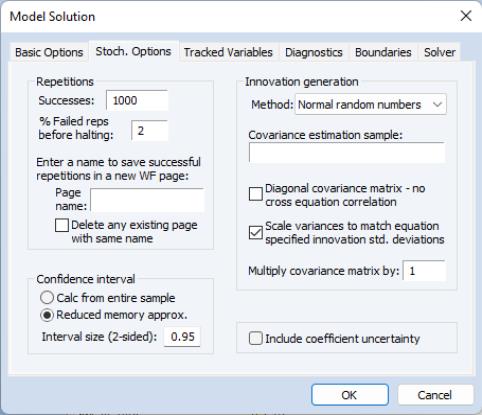
The stochastic options page contains settings used during stochastic simulation. In many cases, you can leave these options at their default settings.
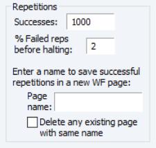
The box, in the top left corner of the dialog, allows you to set the number of repetitions that will be performed during the stochastic simulation. A higher number of repetitions will reduce the sampling variation in the statistics being calculated, but will take more time. The default value of one thousand repetitions is generally adequate to get a good idea of the underlying values, although there may still be some random variation visible between adjacent observations.
Also in the repetitions box is a field labeled . Failed repetitions typically result from random errors driving the model into a region in which it is not defined, for example where the model is forced to take the log or square root of a negative number. When a repetition fails, EViews will discard any partial results from that repetition, then check whether the total number of failures exceeds the threshold set in the box. The simulation continues until either this threshold is exceeded, or the target number of successful repetitions is met.
Note, however, that even one failed repetition indicates that care should be taken when interpreting the simulation results, since it indicates that the model is ill-defined for some possible draws of the random components. Simply discarding these extreme values may create misleading results, particularly when the tails of the distribution are used to measure the error bounds of the system.
The repetitions box also contains a field with the heading: . If a name is provided, the values of the tracked endogenous variables for each successful repetition of the stochastic simulation will be copied into a new workfile page with the specified name. The new page is created with a panel structure where the values of the endogenous variables for individual repetitions are stacked on top of each other as cross sections within the panel. If the checkbox is checked, any existing page with the specified page name will be deleted. If the checkbox is not checked, a number will be appended to the name of the new page so that it does not conflict with any existing page names.
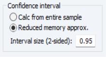
The box sets options for how confidence intervals should be calculated, assuming they have been selected. The Calc from entire sample option uses the sample quantile as an estimate of the quantile of the underlying distribution. This involves storing complete tails for the observed outcomes. This can be very memory intensive since the memory used increases linearly in the number of repetitions. The option uses an updating algorithm due to Jain and Chlamtac (1985). This requires much less memory overall, and the amount used is independent of the number of repetitions. The updating algorithm should provide a reasonable estimate of the tails of the underlying distribution as long as the number of repetitions is not too small.
The box lets you select the size of the confidence interval given by the upper and lower bounds. The default size of 0.95 provides a 95% confidence interval with a weight of 2.5% in each tail. If, instead, you would like to calculate the interquartile range for the simulation results, you should input 0.5 to obtain a confidence interval with bounds at the 25% and 75% quantiles.
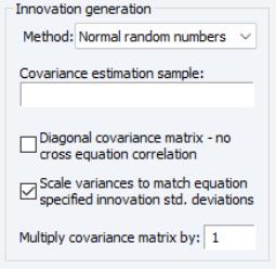
The box on the right side of the dialog determines how the innovations to stochastic equations will be generated. There are two basic methods available for generating the innovations. If is set to the innovations will be generated by drawing a set of random numbers from the standard normal distribution. If is set to the innovations will be generated by drawing randomly (with replacement) from the set of actual innovations observed within a specified sample. Using bootstrapped innovations may be more appropriate than normal random numbers in cases where the equation innovations do not seem to follow a normal distribution, for example if the innovations appear asymmetric or appear to contain more outlying values than a normal distribution would suggest. Note, however, that a set of bootstrapped innovations drawn from a small sample may provide only a rough approximation to the true underlying distribution of the innovations.
When normal random numbers are used, a set of independent random numbers are drawn from the standard normal distribution at each time period, then these numbers are scaled to match the desired variance-covariance structure of the system. In the general case, this involves multiplying the vector of random numbers by the Cholesky factor of the covariance matrix. If the matrix is diagonal, this reduces to multiplying each random number by its desired standard deviation.
The box lets you determine how the variances of the residuals in the equations are determined. If the box is not checked, the variances are calculated from the model equation residuals. If the box is checked, then any equation that contains a specified standard deviation will use that number instead (see
(here) for details on how to specify a standard deviation from the equation properties page). Note that the sample used for estimation in a linked equation may differ from the sample used when estimating the variances of the model residuals.
The box lets you determine how the off diagonal elements of the covariance matrix are determined. If the box is checked, the off diagonal elements are set to zero. If the box is not checked, the off diagonal elements are set so that the correlation of the random draws matches the correlation of the observed equation residuals. If the variances are being scaled, this will involve rescaling the estimated covariances so that the correlations are maintained.
The box allows you to specify the set of observations that will be used when estimating the variance-covariance matrix of the model residuals. By default, EViews will use the default workfile sample.
The field allows you to set an overall scale factor to be applied to the entire covariance matrix. This can be useful for seeing how the stochastic behavior of the model changes as levels of random variation are applied which are different from those that were observed historically, or as a means of trouble-shooting the model by reducing the overall level of random variation if the model behaves badly.
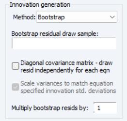
When bootstrapped innovations are used, the dialog changes to show options available for bootstrapping. Similar options are available to those provided when using normal random numbers, although the meanings of the options are slightly different.
The field may be used to specify a sample period from which to draw the residuals used in the bootstrap procedure. If no sample is provided, the bootstrap sample will be set to include the set of observations from the start of the workfile to the last observation before the start of the solution sample. Note that if the bootstrap sample is different from the estimation sample for an equation, then the variance of the bootstrapped innovations need not match the variance of the innovations as estimated by the equation.
The checkbox specifies whether each equation draws independently from a separate observation of the bootstrap sample, or whether a single observation is drawn from the bootstrap sample for all the equations in the model. If the innovation is drawn independently for each equation, there will be no correlation between the innovations used in the different equations in the model. If the same observation is used for all residuals, then the covariance of the innovations in the forecast period will match the covariance of the observed innovations within the bootstrap sample.
The option can be used to rescale all bootstrapped innovations by the specified factor before applying them to the equations. This can be useful for providing a broad adjustment to the overall level of uncertainty to be applied to the model, which can be useful for trouble-shooting if the model is producing errors during stochastic simulation. Note that multiplying the innovation by the specified factor causes the variance of the innovation to increase by the square of the factor, so this option has a slightly different meaning in the bootstrap case than when using normally distributed errors.
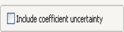
As noted above, stochastic simulation may include both coefficient uncertainty and exogenous variable uncertainty. There are very different ways methods of specifying these two types of uncertainty.
The field at the bottom right of the dialog specifies whether estimated coefficients in linked equations should be varied randomly during a stochastic simulation. When this option is selected, coefficients are randomly redrawn at the beginning of each repetition, using the coefficient variability in the estimated equation, if possible. This technique provides a method of incorporating uncertainty surrounding the true values of the coefficients into variation in our forecast results. Note that coefficient uncertainty is ignored in nonlinear equations and in linear equations estimated with PDL terms.
We emphasize that the dynamic behavior of a model may be altered considerably when the coefficients in the model are varied randomly. A model which is stable may become unstable, or a model which converges exponentially may develop cyclical oscillations. One consequence is that the standard errors from a stochastic simulation of a single equation may vary from the standard errors obtained when the same equation is forecast using the EViews equation object. This result arises since the equation object uses an analytic approach to calculating standard errors based on a local linear approximation that effectively imposes stationarity on the original equation.
To specify exogenous variable uncertainty, you must provide information about the variability of each relevant exogenous variable. First, display the model in variable view by selecting or clicking on the button in the toolbar. Next, select the exogenous variable in question, and right mouse click, select , and enter the exogenous variable variance in the resulting dialog. If you supply a positive value, EViews will incorporate exogenous variable uncertainty in the simulation; if the variance is not a valid value (negative or NA), the exogenous variable will be treated as deterministic.
Tracked Variables
The Tracked Variables page of the dialog lets you examine and modify which endogenous variables are being tracked by the model. When a variable is tracked, the results for that variable are saved in a series in the workfile after the simulation is complete. No results are saved for variables that are not tracked.
Tracking is most useful when working with large models, where keeping the results for every endogenous variable in the model would clutter the workfile and use up too much memory.
By default, all variables are tracked. You can switch on selective tracking using the radio button at the top of the dialog. Once selective tracking is selected, you can type in variable names in the dialog below, or use the properties dialog for the endogenous variable to switch tracking on and off.
You can also see which variables are currently being tracked using the variable view, since the names of tracked variables appear in blue.
Diagnostics
The dialog page lets you set options to control the display of intermediate output. This can be useful if you are having problems getting your model to solve.
When the box is checked, extra output will be produced in the solution messages window as the model is solved.
The traced variables list lets you specify a list of variables for which intermediate values will be stored during the iterations of the solution process. These results can be examined by switching to the view after the model is complete. Tracing intermediate values may give you some idea of where to look for problems when a model is generating errors or failing to converge.
Boundaries
EViews offers the ability to specify boundaries for endogenous variables in a model through a dialog page. Although the solver will not enforce the boundaries while solving the model, EViews will warn you if any variable crosses its boundaries (i.e., solves to a value higher than the upper boundary or less than the lower boundary) for any observation in the solve sample. Boundary violations can also be examined in more detail using the view after the solve is complete.
Solver
You may click on the button on the model toolbar, or select from the main model object menu to display the solution options.
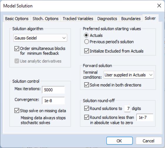
Click on the tab to display the corresponding dialog page. The dialog page sets options relating to the non-linear equation solver which is applied to the model:
The Solution algorithm box lets you select the algorithm that will be used to solve simultaneous blocks within each period and futures values across all periods (if present). The following choices are available:
• : the Gauss-Seidel algorithm is an iterative algorithm, where at each iteration we solve each equation in the model for the value of its associated endogenous variable, treating all other endogenous variables as fixed.
The Gauss-Seidel algorithm requires little working memory and has fairly low computational costs, but requires the equation system to have certain stability properties for it to converge. Although it is easy to construct models that do not satisfy these properties, in practice, the algorithm generally performs well on most econometric models. If you are having difficulties with the algorithm, you may try reordering the equations, or rewriting the equations to change the assignment of endogenous variables, since these changes can affect the stability of the Gauss-Seidel iterations. (See
“Gauss-Seidel”.)
• : Newton's method is an iterative method, where at each iteration we take a linear approximation to the model, then solve the linear system to find a root of the model.
The Newton algorithm can handle a wider class of problems than Gauss-Seidel, but requires considerably more working memory and has a much greater computational cost when applied to large models. Newton's method is invariant to equation reordering or rewriting. (See
“Newton's Method”.)
When this method is selected, Newton's method is used to solve simultaneous blocks but Gauss-Seidel is used to solve future values. (See
“Models Containing Future Values”.)
• : Broyden's method is a modification of Newton's method (often referred to as a quasi-Newton or secant method) where an approximation to the Jacobian is used when linearizing the model rather than the true Jacobian which is used in Newton's method. This approximation is updated at each iteration by comparing the equation residuals obtained at the new trial values of the endogenous variables with the equation residuals predicted by the linear model based on the current Jacobian approximation.
Because each iteration in Broyden's method is based on less information than in Newton's method, Broyden's method typically requires more iterations to converge to a solution. Since each iteration will generally be cheaper to calculate, however, the total time required for solving a model by Broyden's method will often be less than that required to solve the model by Newton's method.
Note that Broyden's method retains many of the desirable properties of Newton's method, such as being invariant to equation reordering or rewriting. (See
“Broyden's Method”.)
When this method is selected, Broyden's method is used to solve simultaneous blocks but Gauss-Seidel is used to solve future values.
• E-Newton: Simultaneous blocks are solved using Broyden's method and future values are solved using Newton's method.
• E-QNewton: Both simultaneous blocks and future values are solved using Broyden's method.
The checkbox controls where EViews takes values for excluded variables. By default, this box is checked and all excluded observations for solved endogenous variables (both in the solution sample and pre-solution observations) are initialized to the actual values of the endogenous variables prior to the start of a model solution. If this box is unchecked, EViews will initialize the excluded variables with values from the solution series (aliased series), so that you may set the values manually without editing the original series.
The checkbox tells the solver to reorder the equations/variables within each simultaneous block in a way that will typically reduce the time required to solve the model. You should generally leave this box checked unless your model fails to converge, in which case you may want to see whether the same behavior occurs when the option is switched off.
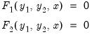
The goal of the reordering is to separate a subset of the equations/variables of the simultaneous block into a subsystem which is recursive conditional on the values of the variables not included in the recursive subsystem. In mathematical notation, if

are the equations of the simultaneous block and

are the endogenous variables:
 | (52.9) |
the reordering is chosen to partition the system into two parts:
 | (52.10) |
where

has been partitioned into

and

and

has been partitioned into

and

.
The equations in

are chosen so that they form a recursive system in the variables in the first partition,

, conditional on the values or the variables in the second partition,

. By a recursive system we mean that the first equation in

may contain only the first element of

, the second equation in

may contain only the first and second elements of

, and so on.
The reordering is chosen to make the first (recursive) partition as large as possible, or, equivalently, to make the second (feedback) partition as small as possible. Finding the best possible reordering is a time consuming problem for a large system, so EViews uses an algorithm proposed by Levy and Low (1988) to obtain a reordering which will generally be close to optimal, although it may not be the best of all possible reorderings. Note that in models containing hundreds of equations the recursive partition will often contain 90% or more of the equations/variables of the simultaneous block, with only 10% or less of the equations/variables placed in the feedback partition.
The reordering is used by the solution algorithms in a variety of ways.
• If the Gauss-Seidel algorithm is used, the basic operations performed by the algorithm are unchanged, but the equations are evaluated in the minimum feedback order instead of the order that they appear in the model. While for any particular model, either order could require less iterations to converge, in practice many models seem to converge faster when the equations are evaluated using the minimum feedback ordering.
• If the Newton solution algorithm is used, the reordering implies that the Jacobian matrix used in the Newton step has a bordered lower triangular structure (it has an upper left corner that is lower triangular). This structure is used inside the Newton solver to reduce the number of calculations required to find the solution to the linearized set of equations used by the Newton step.
• If the Broyden, E-Newton, or E-QNewton solution algorithms are used, the reordering is used to reduce the size of the equation system presented to the Broyden solver by using the equations of the recursive partition to 'substitute out' the variables of the recursive partition, producing a system which has only the feedback variables as unknowns. This more compact system of equations can generally be solved more quickly than the complete set of equations of the simultaneous block.
The checkbox determines whether the solver will take analytic derivatives of the equations with respect to the endogenous variables within each simultaneous block when using solution methods that require the Jacobian matrix. If the box is not checked, derivatives will be obtained numerically.
Analytic derivatives will often be faster to evaluate than numeric derivatives, but they will require more memory than numeric derivatives since an additional expression must be stored for each non-zero element of the Jacobian matrix.
Analytic derivatives must also be recompiled each time the equations in the model are changed. Note that analytic derivatives will be discarded automatically if the expression for the derivative is much larger than the expression for the original equation, as in this case the numeric derivative will be both faster to evaluate and require less memory.
The section lets you select the values to be used as starting values in the iterative procedure. When Actuals is selected, EViews will first try to use values contained in the actuals series as starting values. If actual values are not available, EViews will try to use the values solved for in the previous period. If these are not available, EViews will default to using arbitrary starting values of 0.1. When is selected, the order is changed so that the previous periods values are tried first, and only if they are not available, are the actuals used.
The l section allows you to set termination options for the solver:
• sets the maximum number of iterations that the solver will carry out before aborting.
• sets the threshold for the convergence test. If the largest relative change between iterations of any endogenous variable has an absolute value less than this threshold, then the solution is considered to have converged.
• means that the solver should stop as soon as one or more exogenous (or lagged endogenous) variables is not available. If this option is not checked, the solver will proceed to subsequent periods, storing NAs for this period's results.
The Forward solution section allows you to adjust options that affect how the model is solved when one or more equations in the model contain future (forward) values of the endogenous variables.
• The Terminal conditions section lets you specify how the values of the endogenous variables are determined for leads that extend past the end of the forecast period:
If User supplied in Actuals is selected, the values contained in the Actuals series after the end of the forecast sample will be used as fixed terminal values. If no values are available, the solver will be unable to proceed.
If
Constant level is selected, the terminal values are determined endogenously by adding the condition to the model that the values of the endogenous variables are constant over the post-forecast period at the same level as the final forecasted values (

for
), where

is the first observation past the end of the forecast sample, and

is the maximum lead in the model). This option may be a good choice if the model converges to a stationary state.
If Constant difference is selected, the terminal values are determined endogenously by adding the condition that the values of the endogenous variables follow a linear trend over the post forecast period, with a slope given by the difference between the last two forecasted values:
 | (52.11) |
for

). This option may be a good choice if the model is in log form and tends to converge to a steady state.
If Constant growth rate is selected, the terminal values are determined endogenously by adding the condition to the model that the endogenous variables grow exponentially over the post-forecast period, with the growth rate given by the growth between the final two forecasted values:
 | (52.12) |
for

).
This latter option may be a good choice if the model tends to produce forecasts for the endogenous variables which converge to constant growth paths.
• The Solve in both directions option affects how the solver loops over periods when calculating forward solutions. When the box is not checked, the solver always proceeds from the beginning to the end of the forecast period during the Gauss-Seidel iterations. When the box is checked, the solver alternates between moving forwards and moving backwards through the forecast period.
The two approaches will generally converge at slightly different rates depending on the level of forward or backward persistence in the model. You should choose whichever setting results in a lower iteration count for your particular model.
The section of the dialog controls how the results are rounded after convergence has been achieved. Because the solution algorithms are iterative and provide only approximate results to a specified tolerance, small variations can occur when comparing solutions from models, even when the results should be identical in theory. Rounding can be used to remove some of this minor variation so that results will be more consistent. The default settings will normally be adequate, but if your model has one or more endogenous variables of very small magnitude, you will need to switch off the rounding to zero or rescale the variables so that their solutions are farther from zero.
Solve Control for Target
Normally, when solving a model, we start with a set of known values for our exogenous variables, then solve for the unknown values of the endogenous variables of the model. If we would like an endogenous variable in our model to follow a particular path, we can solve the model repeatedly for different values of the exogenous variables, changing the values until the path we want for the endogenous variable is produced. For example, in a macroeconomic model, we may be interested in examining what value of the personal tax rate would be needed in each period to produce a balanced budget over the forecast horizon.
The problem with carrying out this procedure by hand is that the interactions between variables in the model make it difficult to guess the correct values for the exogenous variables. It will often require many attempts to find the values that solve the model to give the desired results. EViews can address this challenge in two ways. The first is to perform a numerical optimization of the exogenous variable values, automating the search for exogenous values that lead to the desired endogenous values. The second approach respecifies the model in such a way that we can directly solve for the exogenous values.
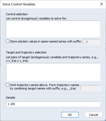
After creating series holding the trajectory values for our endogenous target variables, we can conduct a search for the precipitating values of our exogenous control variables via the item under the model’s menu.
The required parameters are a list of control variables (in the upper text area) and a list of target variables and trajectory series (in the lower text area). These lists may include group objects. The sample over which new control values will be calculated defaults to the current workfile sample. The solved control values will be stored in the original control series by default. The checkbox lets you indicate that the results should be stored in an alternative set of series with the adjoining suffix. This suffix defaults to the active scenario alias suffix, which allows the results to be easily applied to the model via a scenario override. As a convenience, if the trajectory series names are just the target variable names with a suffix applied, you may use the checkbox and adjoining field to shorten the required parameters.
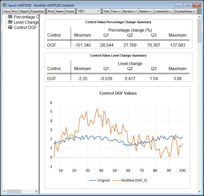
After clicking the button, EViews will determine an appropriate lag for each control variable, conduct the search over control values, and then display a summary of the results in the open model window. The image below shows an example results summary for a single control named DGF.
This summary is a transient rather than a persistent model view and will be lost on the next view change if not frozen.
There are three notable limitations of this numeric approach.
• The model may not contain leads (positive lags).
• There must be an equal number of control and target variables. The overdetermined case with more target variables than control variables is not supported currently.
• The procedure may take some time to complete. Depending on the dependencies among the variables and the control lags selected, the optimization may require multiple bidirectional passes over the sample observations, causing the solution time to be far greater than a standard model solve.
It is also possible for the search to fail, with EViews unable to discovery a set of satisfactory control variable values. You can always alter the control series values (the search’s starting values) and try again.
Endogenous Variable Specification
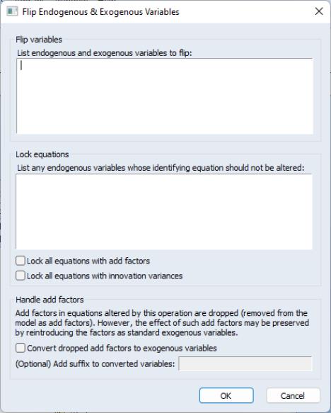
The alternative to a numerical search for exogenous values is to respecify the model such that the exogenous control variables are made endogenous and the endogenous target series are made exogenous. The values of the control series can then be computed using the standard model solve procedure (with the trajectory series overriding the target series). You can automatically rewrite a model’s equations to select a new set of endogenous variables via the item under the model’s menu.
The required parameter is a list of endogenous and exogenous variables to flip (in the upper text area). There must be an equal number of endogenous and exogenous variables (but not add factors) that may be specified in any order. The list may include group objects.
EViews will automatically determine a minimal set of equations to rewrite symbolically. The number of equations rewritten will be at least the number of specified exogenous variables, but could be much greater. If a rewritten equation was included in the model via a linked object, e.g., a VAR, system, or another model, then the link to that object will be broken.
If there are equations that you wish to exclude from being rewritten, you may list the endogenous variable for these “locked” equations in the lower text area. Additionally, you may lock all equations that have associated add factors or innovation variances with the appropriate check box. Naturally, endogenous variables being flipped should not be locked.
Once you click the button, EViews will determine which equations need to be rewritten and then modify the model object accordingly. A summary of the changes made to the model is displayed in the model window.
This approach has several limitations to be aware of:
• Equations containing ARMA specifications will not be altered by this procedure and are treated as locked.
• Currently, all rewritten equations lose their add factors. This deficiency will hopefully be addressed in a future update, but for the time being locking all equations with add factors is the only way to prevent such information loss.
• Rewriting equations is a process of algebraic manipulation, since we are essentially solving equations for a new set of left-hand side variables. Consequently, we are limited by the set of invertible mathematical operations.
It is possible that EViews will be unable to rewrite the model’s equations to produce the desired set of endogenous variables. If you have explicitly locked any equations, you may retry with fewer locked equations, hopefully providing EViews with enough options to be successful.