Estimating Least Squares with Breakpoints in EViews
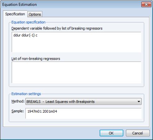
To estimate an equation using least squares with breakpoints, select or from the main EViews menu, then select in the drop-down menu, or simply type the keyword breakls in the command window:
You should enter the dependent variable followed by a list of variables with breaking regressors in the top edit field, and optionally, a list of non-breaking regressors in the bottom edit field.
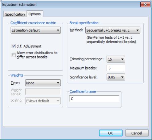
Next, click on the tab to display additional settings for calculation of the coefficient covariance matrix, specification of the breakpoints, weighting, and the coefficient name.
The weighting and coefficient name settings are common to other EViews estimators so we focus on the covariance computation and break specification.
Coefficient Covariance Matrix
The covariance matrix section of the page offers various computation settings.
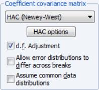
The top drop-down menu should be used to specify the estimator for the coefficient covariances. The is to use the conventional estimator for least squares regression. You may instead elect to use heteroskedasticity robust or covariance calculations. If you specify HAC covariances, EViews will display the button which you may press to bring up a dialog for customizing your calculation.
By default, the covariances will be computed assuming homogeneous errors variances with a common distribution across regimes. You may use the to relax this common distribution restriction.
If you specify either the White or HAC form of robust covariance, EViews will commonly display the checkbox. EViews generally follow Bai and Perron (2003a) who, with one exception, do not impose the restriction that the distribution of the

is the same across regimes. In cases where you employ robust variances, EViews will offer you a choice of whether to assume a common distribution for the data across regimes.
Bai and Perron do impose the homogeneity data restriction when computing HAC robust variances estimators with homogeneous errors. To match the Bai-Perron common error assumptions, you will have to select the .
(Note that EViews does not allow you to specify heterogeneous error distributions and robust covariances in partial breaking models.)
Break Specification
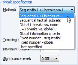
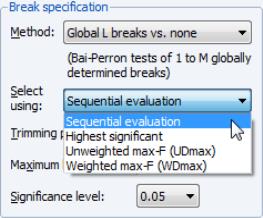
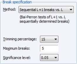
The section of the dialog contains a drop-down where you may specify the type of test you wish to perform. You may choose between:
• Sequential L+1 breaks vs. L
• Sequential tests all subsets
• Global L breaks vs. none
• L+1 breaks vs. global L
• Global information criteria
• Fixed number - sequential
• Fixed number - global
• User-specified
The first two entries determine the optimal number of breaks based on the sequential methodology as described in
“Sequential Determination” above. The methods differ in whether, for a given

breakpoints, we test for an additional breakpoint in each of the

segments (), or whether we test the single added breakpoint that most reduces the sum-of-squares ().
The next three methods employ the global optimizers to determine the number and identities of breaks as described in
“Global Maximization”. If you select one of the global methods, you will see a second drop-down prompting you to specify a sub-method.
• For the method, there are four possible sub-methods. The method chooses the last significant number of breaks, determined sequentially. Selecting chooses the number of breaks that is largest from amongst the significant tests. The latter two settings choose the number of breaks using the corresponding double max test.
• Similarly, if you select the method, a drop-down offers a choice between and .
• The method lets you choose between using the or the .
The next two methods, and , pre-specify the number of breaks and choose the breakpoint dates using the specified method.
The method allows you to specify your own break dates.
Depending on your choice of method, you may be prompted to provide information on one or more additional settings:
• If you specify one of the two fixed number of break methods, you will be prompted for the number of breakpoints (not depicted).
• The
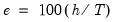
implicitly determines

, the minimum segment length permitted when constructing a test. Small values of the trimming percentage can lead to estimates of coefficients and variances which are based on very few observations.
• The and setting limits the number of breakpoints allowed via global testing, and in sequential or mixed

vs.

testing.
• The drop-down menu should be used to choose between test size values of (0.01, 0.025, 0.05, and 0.10). This setting is not relevant for methods which do not employ testing.
Additional detail on all of the methodologies outlined above is provided in
“Multiple Breakpoint Tests”.