Estimating DiD in EViews
The panel data TWFE model may be estimated using EViews’ built-in estimator for least squares regression with fixed effects. However, EViews also offers a simple interface for estimating the panel TWFE model, featuring tools for performing post-estimation diagnostics such as parallel trends tests, the Goodman-Bacon decomposition and the Callaway-Sant’Anna estimation diagnostic.
(To estimate DiD models on non-panel workfiles, you will need to specify the appropriate least squares model manually using standard least squares regression.)
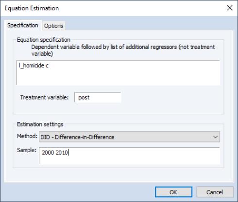
To estimate a DiD model in EViews, bring up the equation dialog by clicking on or from the main menu bar in your panel workfile. EViews will detect the presence of your panel structure and in place of the standard equation dialog will open the panel equation estimation dialog. Select DiD – Difference-in-Difference in the Method dropdown display the DiD dialog:
In the edit field you should enter the dependent variable followed by any exogenous regressors apart from the treatment variable.
The treatment variable should be entered in the edit field. The treatment series should be a binary variable indicating whether the individual has been treated (i.e., is 1 if the observation in a treatment group which is post-treatment date for that group, and 0 otherwise).
The tab contains a single edit field that allows you to change the default coefficient vector.
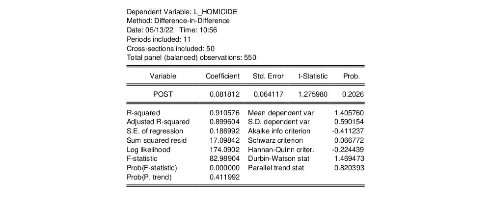
Click on to perform the difference-in-difference estimation and display the output:
The basic equation output for a DiD estimation is identical to that of least squares estimation, but with the display of only the single treatment coefficient. Also, the test statistic and associated p-value of a test of the parallel trends assumption is displayed with the summary statistics at the bottom of the estimation. This test is a simple Wald-test run on the auxiliary regression:
 | (56.6) |
where

is a trend term, and the test evaluates

.
It should also be noted that when performing difference-in-difference estimation, EViews uses cross-section cluster-robust standard errors.
Post-Estimation Views and Procs
Since the TWFE model of DiD is a simple regression model, the standard views and procs available for least squares models are also available for DiD estimation.
There are a set of DiD specific views available under the view menu entry.
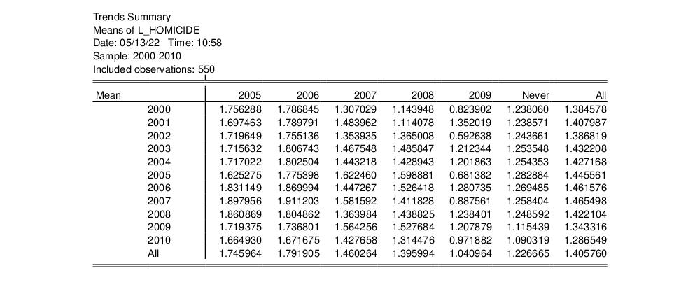
Trends Summary
The and views display the average of the outcome variable by year, categorized by treatment group (i.e., the date at which treatment occurs).
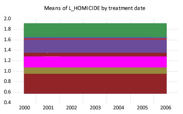
This trends summary graph offers a quick visual representation of the means by treatment group to check whether the different groups have similar trends.
Goodman-Bacon Decomposition
Recent research has noted that the TWFE model is not suitable in multiple-timing DiD models if the impact of treatment changes as time from treatment increases. In this case, the TWFE estimator will exhibit bias since using observations from an already-treated group as the comparison violates the parallel trends assumption.
The view calculates the treatment effects for individual pairs of treatment groups. By focusing on results for different categories of comparisons, the Goodman-Bacon decomposition looks for the presence of parallel trends bias in the computation of the multiple-timing TWFE.
Goodman-Bacon (2021) shows that the TWFE estimator is a weighted average of DiD estimators for every combination of two groups of observations defined by two treatment dates (

comparisons). The weights used in the average are based upon the number of observations and the variance of the estimated treatment effect in these individual DiD comparisons.
Specifically, for every treatment group with a given treatment date (group

), we compute all

comparisons with:
• observations treated at later dates (

groups)
• observations treated at earlier dates (

groups)
• never treated observations (group

)
• always treated observations (group

)
For the first set of cases where

is an early treatment group (

) compared with a later group (

), we employ only
untreated 
observations from periods up to the beginning of the treatment date, so that the

can serve as a non-changing control.
For the second set of cases where

is a later treatment group (

) compared with an earlier group (

), we employ only
treated 
observations from periods following the treatment date, so that the

can serve as a non-changing control.
It is important to note that both the

against

, and the

against

comparisons employ control groups that consist of previously treated observations. These comparisons are particularly susceptible to parallel trends bias when the treatment effect varies from the date of treatment.
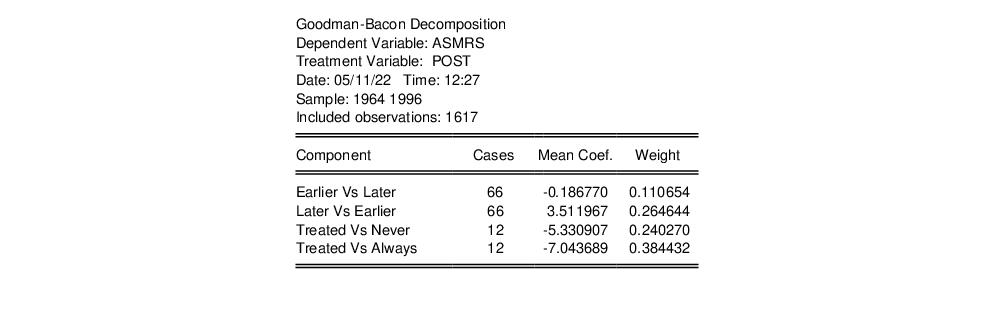
To display the decomposition, click on . EViews will display a spool view of output divided into three sections.
The first section shows weighted means of the treatment effect categorized by the type of

group comparison:
The column shows the number of year pairs used in the comparison. In this example, there are 66 treatment date pairs in which

and untreated

observations are compared, and 12 years in which both the

and

observations are compared with the

observations.
The column the estimate of the ATET, while the column contains the weights used in forming the overall ATET estimate. Here the estimated ATET across

vs. untreated

comparisons is -0.1868 with a weight of 0.1107. The estimated ATET for the

and

observations vs.

observations is -7.0437, with a weight of 0.3844.
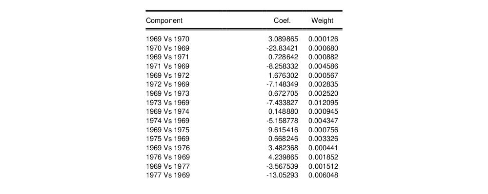
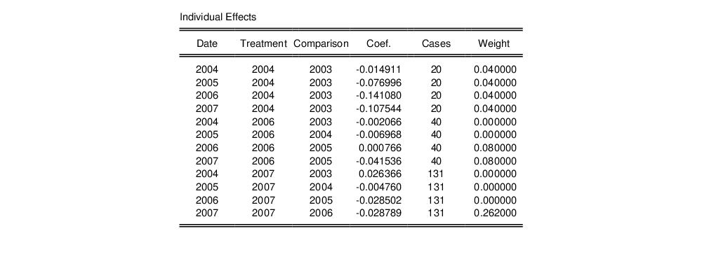
Each of the ATET components in this table is itself a weighted average of individual treatment-year pair comparisons. The second section of the spool displays the individual

coefficient estimates and weights for every comparison. For example, the first few lines of a Goodman-Bacon decomposition are given by:
The labeling of the individual components indicates the nature of the group comparison. For example, the “1969 vs. 1970” comparison is an

against

comparison, while the “1970 vs. 1969” is the

against

comparison.
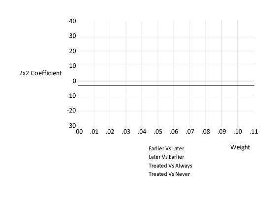
The final section in the spool contains a graph of the individual

component results, with different symbols and colors indicating the type of comparison. The graphical representation of the individual effects shown in the third section allows a quick visualization of the effects:
Group-Time Effects (Callaway-Sant’Anna)
The Group-Time Average Treatment Effects (Callaway-Sant’Anna) view computes the Callaway and Sant’Anna (2021) estimator of the average treatment effects.
A study by Callaway and Sant’Anna (2020, CS) derives a new estimator for the DiD model with multiple treatment time periods, breaking away from the TWFE estimator by using weighted averages of the differences model
Equation (56.1) with appropriate comparison pairings.
Their estimator is robust to the treatment effect changing as time from treatment increases so that the CS estimator can be useful as a diagnostic comparison to the TWFE estimator to judge the reliability of the TWFE estimates.
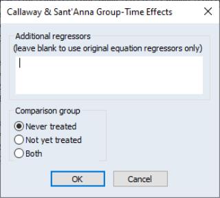
To display the view select from the equation menu. EViews displays a dialog:
• The Additional regressors edit field allows you to estimate the Callaway and Sant’Anna model on the underlying estimated TWFE model, but with additional regressors. This allows you to estimate models via Callaway and Sant’Anna that may be impossible to estimate via TWFE due to perfect collinearity. Simply enter the name of series, or series expressions, you wish to add to the estimation in the edit field.
By default the CS estimator compares treated individuals grouped by treatment date against a control group of individuals who never receive treatment. However these comparisons could be modified to include individuals who have not yet been treated as the control group.
Each pairing compares groups the treated into year-of-treatment groups, and then compares the difference between the output variable in each year after treatment with the year prior to treatment. This difference is compared for the treatment group and the comparison group.
• The Comparison group radio buttons specify whether the comparison/control groups in the Callaway-Sant’Anna model will be only those individuals who never receive treatment (Never treated), or those who have yet to receive treatment in the current time period (Not yet treated), or either (Both).
Clicking OK will estimate the Callaway and Sant’Anna model. The output is in the form of a spool with five sections.
The first section provides a summary view of the CS results, including the overall average treatment effect of the treated (calculated as the weighted average of the individual pairing calculations), along with its standard-error, z-statistic and associated p-value.
The second section provides each of the individual pairings used in the weighted average ATET estimation, including the estimated coefficient for the pairing, and its weight.
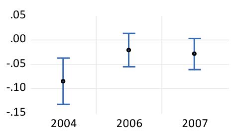
The remaining sections computes aggregations of the individual pairings, where the aggregations are over treatment date (group), observation date (date), and time-since treatment (duration). For each aggregation, the coefficients, standard errors, z-Statistics and associated p-values are tabulated, along with a graph of the coefficients and a 95% confidence interval.
For example, the group effects consist of the weighted averages of the ATET coefficients
and the corresponding plot
shows the values along with 95% confidence intervals
Borusyak, Jaravel, and Spiess Imputed Estimator
A third study by Borusyak, Jaravel and Spiess (2021, BJS) describes a number of potential issues with the TWFE estimator and derives an estimator that alleviates these issues. They term their estimator an “imputation” estimator, since it uses estimates from untreated observations to forecast the outcome variable for observations for which individuals have been treated, and then for each treated observation they impute the impact of treatment as the difference between the forecast of the outcome, and the observed outcome. This series of differences can then be averaged over to compute the average treatment effect.
To display the view select from the equation menu.
EViews estimates the BJS estimator and displays the output in a spool. As with the Group-Time Effects view (
“Group-Time Effects (Callaway-Sant’Anna)”), there are five sections in the output: the summary view with the overall ATET, its standard-error,
z-statistic and associated
p-value, the individual pairings used in the weighted average ATET estimation, and sections for aggregations over treatment date (group), observation date (date), and time-since treatment (duration).
Make Underlying Equation Proc
One additional DiD-specific tool is the proc. Clicking on will produce a new equation object in which the difference-in-difference model as a standard least squares equation. Having an equation with the DiD specification estimated by least squares may prove useful for performing diagnostics or additional analysis.