Examples
To demonstrate the use of DiD estimation in EViews we will replicate results from familiar papers.
Card and Krueger (1994)
We first replicate results from one of the most famous DiD studies, the Card and Krueger (1994) paper analyzing the impact of minimum wage laws on employment in fast food workers.
Although Card and Krueger’s study is involves difference-in-difference estimation, they only have two time periods: February/March 1992 and November/December 1992. They term these two periods Wave 1 and Wave 2. During the gap between these two periods, New Jersey increased the state minimum wage from $4.25 to $5.05. Pennsylvania, a neighboring state, maintained its minimum wage at $4.25 during the same time period.
A subset of the data used in this paper are available in the workfile “CardKrueger.wf1”. The data in the workfile contain data for 410 fast-food restaurants, 331 in New Jersey and 79 in Pennsylvania. There are three series containing employment data: EMPFT has the number of full time employees in each store, EMPTOT has the total number of employees, and EMPTOTC has the total number of employees, with stores that have closed down coded as a 0 (instead of an NA). The series HRSOPEN contains the number of hours, per day, each store is open. The NEWMIN series is a binary variable indicating whether a store is subject to an increased in the minimum wage (i.e. is based in New Jersey during wave 2).
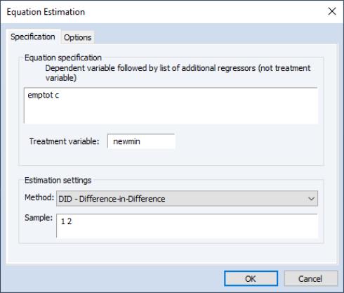
We can replicate one of the results in the Card and Krueger paper by performing a simple difference-in-difference estimation of EMPTOT against NEWMIN. We click on and then selectfrom the dropdown to display the dialog:
Enter “EMPTOT C” in the edit field, the name of the treatment indicator “NEWMIN” in the edit field, and “1 2” in the edit field. Click on to estimate this specification. EViews will display the estimation results:
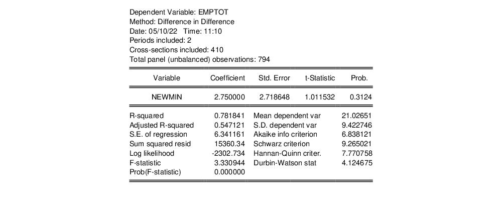
The estimate of the impact of the increase in the minimum wage on employment is 2.75. This matches the result in Row 4., column (iii) of Table 3 in Card and Krueger, and forms part of the basis for their overall finding that raising the minimum wage in New Jersey actually led to an increase in employment.
As noted earlier, the standard error of the estimate and the t-statistic p-value employ cross-section cluster-robust standard error calculations.
Note the test statistic and p-value for the parallel trends test are not displayed at the bottom of the table, since with only two time periods, an estimate of trend values cannot be computed.
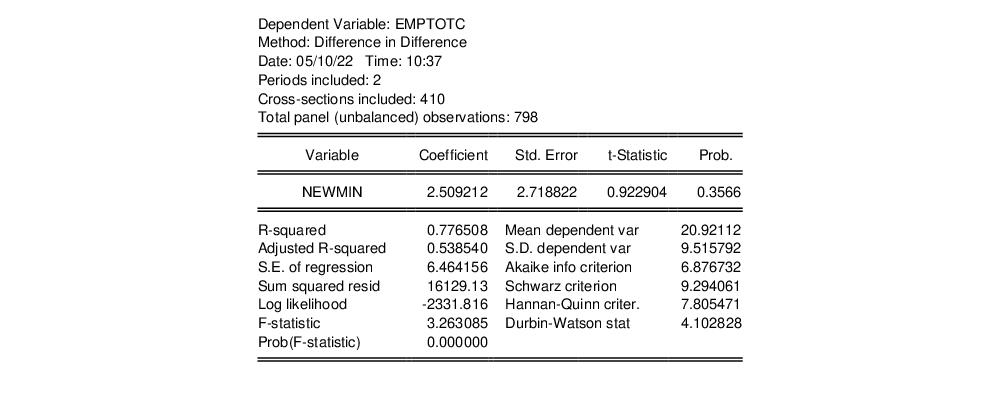
If we use EMPTOTC as the outcome variable instead of EMPTOT, we can replicate the result in Row 5, column (iii) of Table 3 in Card and Krueger, which reports that the impact of the raise in minimum wage is 2.51.
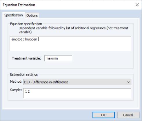
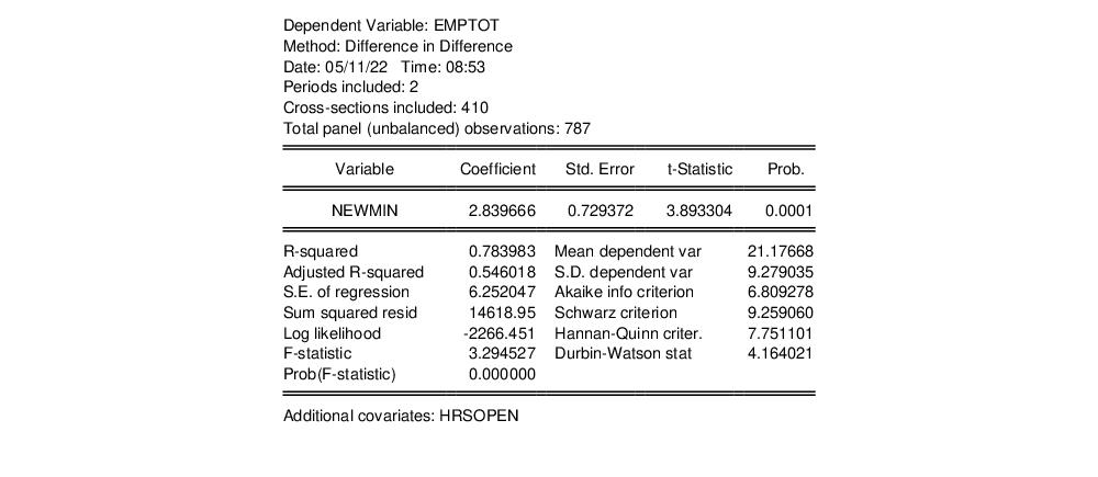
We could extend the specification to include the number of hours a store is open as a covariate, simply by entering “HRSOPEN” as a regressor in the edit field:
Although not a specification estimated by Card and Krueger, estimation results for the extended model allow evaluation of whether the basic result is sensitive to inclusion of this covariate.
Click on OK to estimate the expanded specification. The results are given by:
We can see that the inclusion of the HRSOPEN covariate (which is indicated at the bottom of the output) did not have a large impact on the estimate of the effect of the minimum wage increase (2.84 compared with the original 2.75), though the statistical significance of the result is enhanced considerably.
Stevenson and Wolfers (2006)
As a second example, we will first replicate the study by Stevenson and Wolfers (2006), which analyzed the impact of the introduction of no-fault divorce reforms on female suicide rates. The dependent variable consists of annual suicide rates for US states between 1964 and 1996. Throughout this period a number of states, at different times, introduced no-fault divorce reform.
This paper and the corresponding data was also studied by Goodman-Bacon (2021) as an application of the Goodman-Bacon decomposition.
A subset of the data used in Stevenson and Wolfers is available in Stata format from Austin Nichols’
website. We can easily open this file in EViews, and EViews will automatically detect the panel nature of the data and set up the workfile with that structure:
The file contains data on the female suicide mortality rate in the series ASMRS, a binary series, POST, equal to 1 if an observation is in a no-fault divorce environment, and zero if no-fault divorces are not allowed, as well as cross-section (state) and date (year) series.
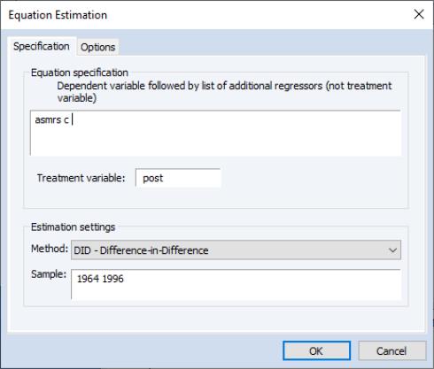
To determine the impact of no-fault divorce reform on female suicide mortality rate we can perform a simple difference-in-difference, with multiple timings, estimation. We click on and then change the dropdown to . Note this method is only available because we have a workfile structured as a panel. We enter “ASMRS” as the dependent/outcome variable, followed by our treatment dummy, “POST”, and the sample pair “1964 1996”:
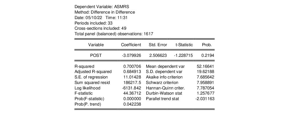
Clicking produces the estimation output:
The estimate of the impact of no-fault divorce reform on suicide mortality in females is -3.08, which matches the number presented in Section III of Goodman-Bacon (2021).
To view the Goodman-Bacon decomposition (
“Goodman-Bacon Decomposition”) we click on :
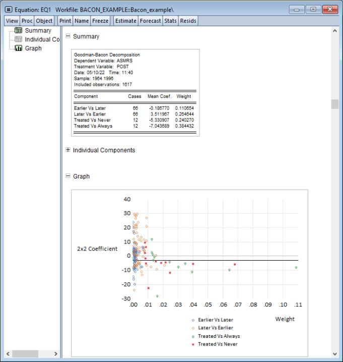
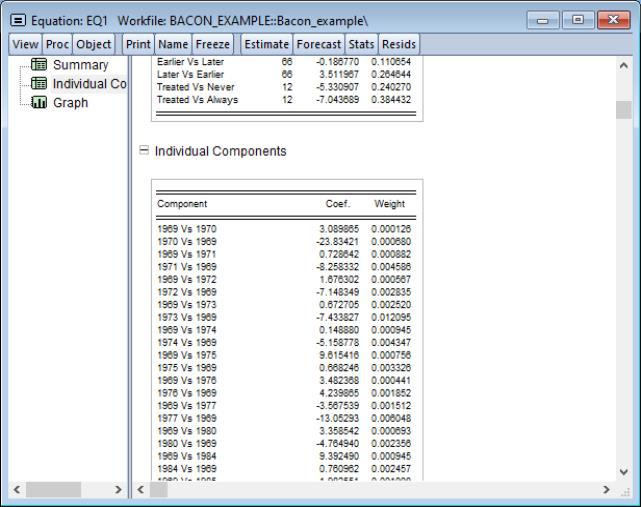
EViews opens a spool with output divided into three sections. The middle section showing all of the

individual coefficients and weights for each pair of treatment dates is closed by default. These individual results can be displayed by clicking the “+” symbol:
We can see that the

coefficient comparing observations that introduced divorce reform in 1969 with those that introduced reform in 1970 is 3.09.
The weighted average of these individual year pair-comparisons, combined into groups, is displayed in the first section. We can see that each of the groupings has a negative coefficient, apart from the “Later vs. Earlier” group. Since this comparison group may violate the parallel trends assumption, it is possible that a biased positive coefficient with large weight may have upwardly biased the overall TWFE coefficient to the reported value of -3.08.
We can see that there is a large number of the “Later vs. Earlier” group above the overall estimated coefficient, again indicating that this group may be upwardly biasing the overall estimate.
Callaway and Sant’Anna (2021)
As a third example, we’ll examine the data used in Callaway and Sant’Anna (2021). Similar to the Card and Krueger (1994_, Callaway and Sant’Anna study the impact of the minimum wage on employment levels, but this time concentrating on teen employment. The data contains county level teen employment between 2003–2007. During this time period the federal minimum wage remained constant at $5.15 per hour. However some states increased the minimum wage within the state above the federal level during the time period. Counties within such states are the treated group (with different treatment times). Counties within states that did not change their minimum wage are in the control group.
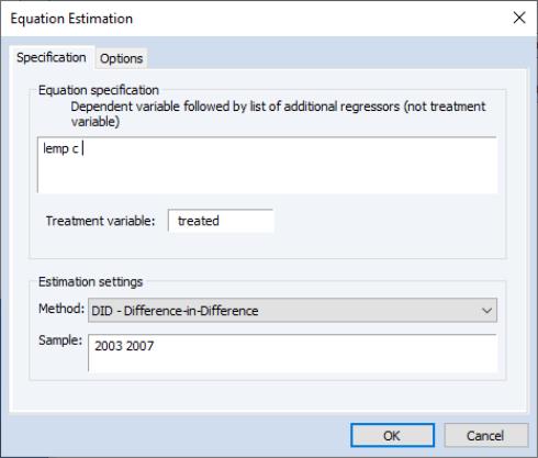
These data are provided in the workfile “CallawaySantanna.wf1”. The series TREATED is a binary variable indicating whether a county has been subject to an increased minimum wage in the time period, the series LEMP contains the log of employment for that county in that time period, and the series LPOP contains the log of the population within the county. A TWFE estimation of the impact of minimum wage on employment can be performed by clicking on and then changing the dropdown to . We enter “LEMP” as the dependent/outcome variable, followed by our treatment dummy, “TREATED”, and sample pair “2003 2007”:
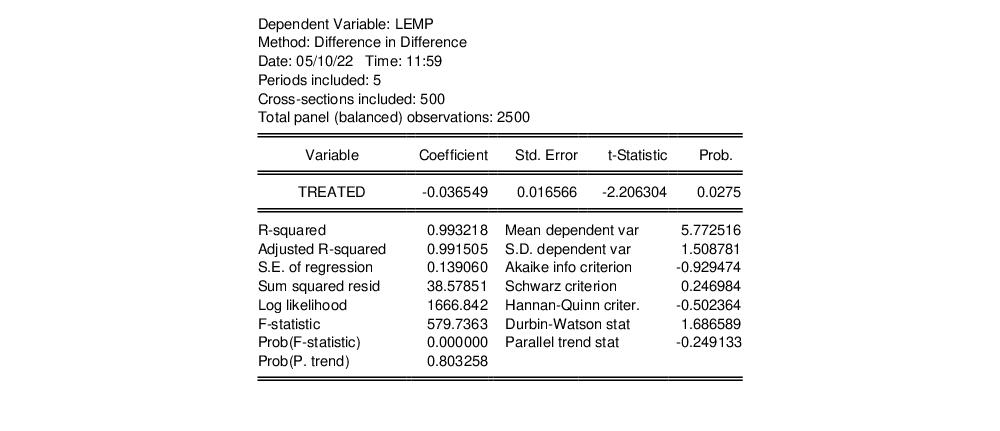
Click on to estimate the specification:
Note the TWFE estimate of the impact of treatment matches that given in Callaway and Sant’Anna, Table 3, section A.
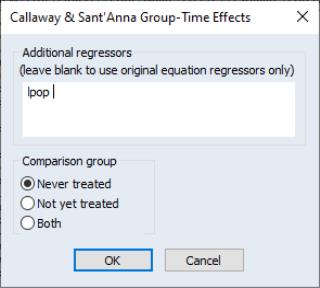
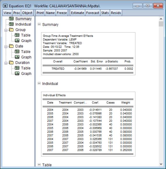
To view the Callaway-Sant’Anna estimator we click on CS Group-Time Effects… which brings up the Callaway-Sant’Anna dialog:
Note, we’ll include an additional regressor, LPOP, and set the comparison group to by those states who never perform divorce reform. Since county population is constant through the time period being analyzed (population data is taken from the 10 year census), it would not be possible to include it as an explanatory variable in TWFE estimation. However, it may be used in the CS estimator.
The top portion of the output displays the overall estimate of the treatment effect, -0.042, which compares with the TWFE estimate of -0.37.
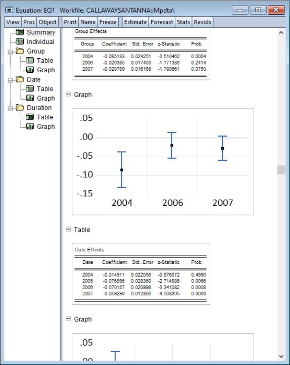
Below this section we can see the individual coefficients for each date pairing, as well as aggregations of them by treatment date (Group), observation date (Date) and time-since-treatment (Duration).