Exponential Smoothing
Exponential smoothing is a simple method of adaptive forecasting. It is an effective way of forecasting when you have only a few observations on which to base your forecast. Unlike forecasts from regression models which use fixed coefficients, forecasts from exponential smoothing methods adjust based upon past forecast errors. For additional discussion, see Bowerman and O’Connell (1979).
EViews offers two methods of performing exponential smoothing: simple exponential smoothing based on older ad hoc methods, and exponential smoothing based on the Error-Trend-Seasonal likelihood framework of Hyndman, Koehler, et al. (2002).
Simple Exponential Smoothing
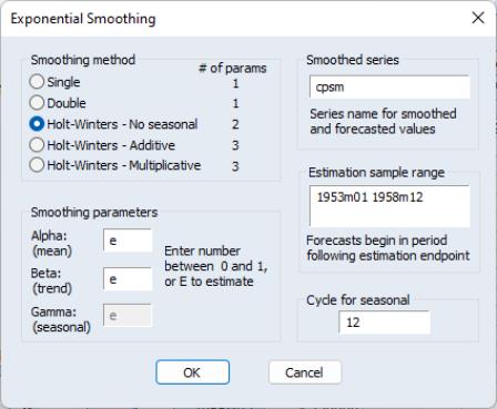
To obtain forecasts based on exponential smoothing methods, choose . The dialog box appears:
You need to provide the following information:
• Smoothing Method. You have the option to choose one of the five methods listed.
• Smoothing Parameters. You can either specify the values of the smoothing parameters or let EViews estimate them.
To estimate the parameter, type the letter e (for estimate) in the edit field. EViews estimates the parameters by minimizing the sum of squared errors. Don't be surprised if the estimated damping parameters are close to one—it is a sign that the series is close to a random walk, where the most recent value is the best estimate of future values.
To specify a number, type the number in the field corresponding to the parameter. All parameters are constrained to be between 0 and 1; if you specify a number outside the unit interval, EViews will estimate the parameter.
• Smoothed Series Name. You should provide a name for the smoothed series. By default, EViews will generate a name by appending SM to the original series name, but you can enter any valid EViews name.
• Estimation Sample. You must specify the sample period upon which to base your forecasts (whether you choose to estimate the parameters or not). The default is the current workfile sample. EViews will calculate forecasts starting from the first observation after the end of the estimation sample.
• Cycle for Seasonal. You can change the number of seasons per year from the default of 12 for monthly or 4 for quarterly series. This option allows you to forecast from unusual data such as an undated workfile. Enter a number for the cycle in this field.
Single Smoothing (one parameter)
This single exponential smoothing method is appropriate for series that move randomly above and below a constant mean with no trend nor seasonal patterns. The smoothed series

of

is computed recursively, by evaluating:
 | (11.54) |
where

is the
damping (or
smoothing) factor. The smaller is the

, the smoother is the

series. By repeated substitution, we can rewrite the recursion as
 | (11.55) |
This shows why this method is called exponential smoothing—the forecast of

is a weighted average of the past values of

, where the weights decline exponentially with time.
The forecasts from single smoothing are constant for all future observations. This constant is given by:
 | (11.56) |
where

is the end of the estimation sample.
To start the recursion, we need an initial value for

and a value for

. EViews uses the mean of the initial

observations of

to start the recursion (where

is the number of observations in the sample). Bowerman and O’Connell (1979) suggest that values of

around 0.01 to 0.30 work quite well. You can also let EViews estimate

to minimize the sum of squares of one-step forecast errors.
Double Smoothing (one parameter)
This method applies the single smoothing method twice (using the same parameter) and is appropriate for series with a linear trend. Double smoothing of a series

is defined by the recursions:
 | (11.57) |
where

is the single smoothed series and

is the double smoothed series. Note that double smoothing is a single parameter smoothing method with damping factor

.
Forecasts from double smoothing are computed as:
 | (11.58) |
The last expression shows that forecasts from double smoothing lie on a linear trend with intercept

and slope

.
Holt-Winters—Multiplicative (three parameters)
This method is appropriate for series with a linear time trend and multiplicative seasonal variation. The smoothed series

is given by,
 | (11.59) |
where
 | (11.60) |
These three coefficients are defined by the following recursions:
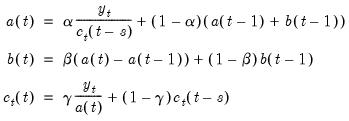 | (11.61) |
where

are the damping factors and

is the seasonal frequency specified in the
Cycle for Seasonal field box.
Forecasts are computed by:
 | (11.62) |
where the seasonal factors are used from the last

estimates.
Holt-Winters—Additive (three parameter)
This method is appropriate for series with a linear time trend and additive seasonal variation. The smoothed series

is given by:
 | (11.63) |
where

and

are the permanent component and trend as defined above in
Equation (11.60) and

are the additive seasonal factors. The three coefficients are defined by the following recursions:
 | (11.64) |
where

are the damping factors and

is the seasonal frequency specified in the
Cycle for Seasonal field box.
Forecasts are computed by:
 | (11.65) |
where the seasonal factors are used from the last

estimates.
Holt-Winters—No Seasonal (two parameters)
This method is appropriate for series with a linear time trend and no seasonal variation. This method is similar to the double smoothing method in that both generate forecasts with a linear trend and no seasonal component. The double smoothing method is more parsimonious since it uses only one parameter, while this method is a two parameter method. The smoothed series

is given by:
 | (11.66) |
where

and

are the permanent component and trend as defined above in
Equation (11.60).
These two coefficients are defined by the following recursions:;
 | (11.67) |
where

are the damping factors. This is an exponential smoothing method with two parameters.
Forecasts are computed by:
 | (11.68) |
These forecasts lie on a linear trend with intercept

and slope

.
It is worth noting that Holt-Winters—No Seasonal, is
not the same as additive or multiplicative with

. The condition

only restricts the seasonal factors from changing over time so there are still (fixed) nonzero seasonal factors in the forecasts.
Illustration
As an illustration of forecasting using exponential smoothing we forecast data on monthly housing starts (HS) for the period 1985m01–1988m12 using the DRI Basics data for the period 1959m01–1984m12. These data are provided in the workfile “Hs.WF1”. Load the workfile, highlight the HS series, double click, select . We use the method to account for seasonality, name the smoothed forecasts HSSM, and estimate all parameters over the period 1959m1–1984m12. Leave the remaining settings at their default values.
When you click OK, EViews displays the results of the smoothing procedure. The first part displays the estimated (or specified) parameter values, the sum of squared residuals, the root mean squared error of the forecast. The zero values for Beta and Gamma in this example mean that the trend and seasonal components are estimated as fixed and not changing.
The second part of the table displays the mean

, and trend

at the end of the estimation sample that are used for post-sample smoothed forecasts.
For seasonal methods, the seasonal factors

used in the forecasts are also displayed. The smoothed series in the workfile contains data from the beginning of the estimation sample to the end of the workfile range; all values after the estimation period are forecasts.
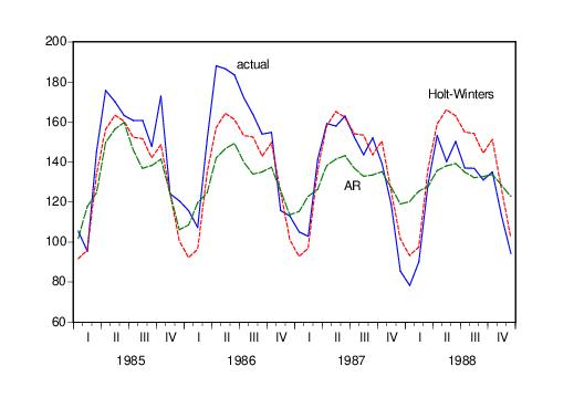
When we plot the actual values (HS) and the smoothed forecasts (HSSM) on a single graph, we get:
We have included the forecasted values HSF from estimation of an AR model with an AR(1) and a SAR(12) term for comparison purposes. The forecasts from the multiplicative exponential smoothing method do a better job of tracking the seasonal movements in the actual series.
ETS Exponential Smoothing
Although ad hoc exponential smoothing (ES) methods have been employed for many decades, recent methodological developments have embedded these models in a modern dynamic nonlinear model framework (see Chatfield, et al. 2001 for a brief historical overview).
Hyndman, Koehler, et al. (2002) outline the ETS (Error-Trend-Seasonal or ExponenTial Smoothing) framework which defines an extended class of ES methods and offers a theoretical foundation for analysis of these models using state-space based likelihood calculations, with support for model selection and calculation of forecast standard errors.
Notably, the ETS framework encompasses the standard ES models (e.g., Holt and Holt–Winters additive and multiplicative methods), so that it provides a theoretical foundation for what was previously a collection of ad hoc approaches.
The remainder of this section outlines briefly the basics of ETS exponential smoothing models and describes their estimation in EViews. Users who desire additional detail should consult Ord, Koehler, and Snyder (1997), Hyndman, Koehler, Snyder, and Grose (2002), and in particular, the book-length treatment by Hyndman, Koehler, Ord, and Snyder (2008).
ETS Decomposition
The time series

may be decomposed into three components, trend (T), seasonal (S), and error (E), where the trend term characterizes the long-term movement of

, the seasonal term corresponds to a pattern with known periodicity, and the error term is the irregular, unpredictable component of the series.
These three components may be combined in various additive and multiplicative combinations to produce

. We may have a purely additive model, say

or

, a pure multiplicative model like

or

, or models which mix the two, as in

or

The individual components of an ETS specification may be specified as being of the form:
 | (11.69) |
where N = none, A = additive, M = multiplicative, AD = additive dampened, and MD = multiplicative dampened (damping uses an extra parameter to reduce the impact of the trend over time). The are a total of

possible ETS models associated with these choices.
The trend specification requires a bit of additional discussion. The forecasted trend term

may itself be decomposed into a level term (

) and a growth term (

) in several ways. Following Hyndman,
et al. (2008) we let

be the trend forecast

periods out, and let

be a damping parameter. The five different trend types corresponding to different assumptions about the growth term are given by:
None | |
Additive | |
Additive damped | |
Multiplicative | |
Multiplicative damped | |
for

.
ETS Representation
We have seen that the trend is comprised of a level term (

) which is always present, and a growth term (

) which may or may be present, depending on the trend specification. If we let

represent included seasonal terms, we may define the general following

-dimensional state vector:
 | (11.70) |
Following Ord, Koehler, and Snyder (1997), we may write a nonlinear dynamic model representation of the exponential smoothing equations using a state space model with a common error term:
 | (11.71) |
where the

and

are known continuous scalar functions,

and

are known continuously functions with continuous derivatives from

and

where

independent of past realizations of

and

.
Conceptually, the

equation represents how the various state variable components

are combined to express the series in terms of a smoothed forecast

and the prediction error

. The multiple functions are a notational device for writing the additive and multiplicative errors in compact form. With additive errors we have

so that
 | (11.72) |
With multiplicative errors we set

, yielding
 | (11.73) |
The

equations outline the process by which the component estimates are updated using the previous period’s estimates and the current prediction error

. For the ETS models considered here, we may think of the updating smoothing equations as being weighted averages of a term which depends on the current prediction error (and prior states), and one which depends on the prior states. The resulting state equations are extended versions of those outlined by Hyndman,
et al. (2002), and take the general form:
 | (11.74) |
where

,

and

are functions of the prediction error and lagged states, and

is a function of the lagged states.

is the damping parameter for linear trend models and

is the damping parameter for multiplicative trend models. In the absence of a damping, the parameters are set to 1.
The exact forms of all of these equations depend on the specific ETS specification. The expressions corresponding to the 30 possible specifications are listed in Hyndman, et al. (2008, Tables 2.2 and 2.3, p. 21–22). We do not reproduce the results here, but instead offer examples to show how familiar models fit into the framework.
Simple Exponential Smoothing (A, N, N)
To take the simplest example, consider the simple exponential smoothing (A,N,N) specification. For this model, the contemporaneous estimate of the level may be written as the weighted average of the current value of the variable and its forecasted value:
 | (11.75) |
where the forecast is the previous value of the state,

. For this linear error specification, obtain the prediction error equation
 | (11.76) |
Substituting for

and

in
Equation (11.75), we have an updating equation in error correction form:
 | (11.77) |
The full model may be written in ETS form as (Hyndman, et al., 2008, Table 2.2, p. 21):
 | (11.78) |
This specification is an ETS model defined by
Equation (11.72) and
Equation (11.74) with state

, and functions

,

, and

.
Holt’s Method with Multiplicative Errors (M, A, N)
Next, consider Holt’s linear trend method with multiplicative errors (M, A, N). Define the state vector

and let

be the one-period ahead forecast of

since we have an additive trend specification with no seasonal component.
Given this forecast, the multiplicative error assumption implies that:
 | (11.79) |
The updating equation for the level state variable is obtained by forming a weighted average of the previous period component and a term which depends on the prediction error. We have
 | (11.80) |
so that

and

.
Similarly, for the growth component, we have
 | (11.81) |
so that

and

.
The ETS representation for this model may be written as:
 | (11.82) |
(Hyndman, et al., 2008, Table 2.3, p. 22.)
Holt-Winters Method with Multiplicative Errors and Seasonals (M, A, M)
Consider the Holt-Winters (M, A, M) linear trend model with multiplicative errors and multiplicative seasonal (

). Define the state vector

. The one-period ahead forecast is
 | (11.83) |
and the prediction error decomposition is
 | (11.84) |
The level state equation is given by the weighted average of a term involving the prediction error and the previous state forecast:
 | (11.85) |
Similarly, the growth equation is
 | (11.86) |
and the seasonal equation is
 | (11.87) |
The ETS representation for the (M, A, M) model is then:
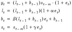 | (11.88) |
(Hyndman, et al. 2008, Table 2.3, p. 22).
Fully Multiplicative Method with Damping (M, Md, M)
Consider an damped exponential trend model with multiplicative seasonal and error components (M, Md, M). Define the state vector

and let

be the one-period ahead forecast of

. Then the prediction error decomposition is
 | (11.89) |
The level state equation is given by:
 | (11.90) |
The growth equation is
 | (11.91) |
Notice that this state equation is of the form in
Equation (11.74) with

(since we have a multiplicative damped trend) and

.
The seasonal equation is
 | (11.92) |
![]() | (11.93) |
Then the ETS representation for the (M, Md, M) model is:
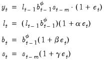 | (11.94) |
(Hyndman, et al. 2008, Table 2.3, p. 22).
Parameters and Initial States
Given any ETS specification, parameters

, and values for the initial states

, we may use the ETS state and prediction equations to obtain smoothed estimates of the unobserved components and the underlying series. Typically the parameters are estimated. The initial states are either estimated or assigned
ad hoc values.
Some ETS models require only a subset of the parameters and states. Models without a seasonal component, for example, use neither the seasonal parameter

, nor the initial seasonal states

. We will use

and

to refer to the relevant subsets for a given model which are to be estimated.
Parameters
The parameter values are usually unknown and must be estimated. There have been many suggestions for reducing the size of the potential parameter space for

. The traditional approach has assigned the following restrictions on the parameters to ensure model stability:
 | (11.95) |
Initial states
Traditionally, the initial state values are specified using ad hoc values. The ETS approach allows for either the use of these experimental values, or estimation of the initial states as part of the optimization problem. Even when the initial states are estimated, it is useful to use ad hoc values as a starting point for optimization.
Following Hyndman, et al. (2002) EViews uses the following ad hoc method for computing the initial states or starting values for the estimated initial states:
• Initial level components: For nonseasonal data, compute a linear trend on the first ten observations against a time series

. For seasonal data, compute a linear trend using linear regression on the first ten seasonally adjusted values against a time series. And then set the initial level

to be the intercept of the trend.
• Initial growth components: For additive trends, set

to be the slope of the trend. For multiplicative trends, set

where

and

denote the intercept and slope of the fitted trend, respectively.
• Initial seasonal component: Compute a

moving average through the first few years of data. Denote this set of values

. For additive seasonality, detrend the data to obtain

. For multiplicative seasonality, detrend the data to obtain

. Compute initial seasonal indices

by averaging the detrended data for each season. Normalize these seasonal indices so that they add to zero for additive seasonality, and add to

for multiplicative seasonality.
Estimation
EViews offers both maximum likelihood (ML) and average mean square error minimization (AMSE) methods of estimating the unknown parameters

and, optionally, the initial states

.
Maximum Likelihood Estimation
The maximum likelihood estimator finds the parameters and initial states that maximize the log-likelihood function. The Gaussian log-likelihood for ETS specifications can be written in terms of the prediction errors as
 | (11.96) |
For a given set of parameters and initial states and ETS model, the likelihood is evaluated recursively using the state equations and solving for the prediction error using the appropriate prediction decomposition equation.
The parameters and initial conditions are obtained by maximizing the likelihood in
Equation (11.96) with respect to

,

, and

using the Broyden, Fletcher, Goldfarb and Shanno (BFGS) algorithm.
Average Mean Square Error Minimization
The average mean square error estimator finds the parameter values and initial state values that minimize the average mean square error of the

-step forecasts of the specified ETS model.
Recall that our prediction error is simply the one-step ahead forecast error for the series:

. The

-step ahead forecast error is defined as
 | (11.97) |
where the components of

are obtained by recursively solving the state equations assuming

in each period.
The average mean square error of the

-step forecasts is defined as
 | (11.98) |
The AMSE is then minimized with respect to the

and

using BFGS.
For example, for the (M, A, N) specification described earlier (
“Holt’s Method with Multiplicative Errors (M, A, N)”), and

we have
 | (11.99) |
so that

, and
 | (11.100) |
so that

. Then the

-step ahead forecasts are
 | (11.101) |
The AMSE is then given by
 | (11.102) |
Model Selection
The ETS smoothing framework lends itself to automatic model selection. Since both a likelihood and a forecast error can be calculated for each ETS model it is possible to compare a likelihood based information criterion or out-of-sample AMSE across models to determine which one more closely fits the data (using the likelihood), or forecasts more accurately (using AMSE).
Likelihood based comparisons can be performed using the standard likelihood based criteria: Akaike Information Criterion (AIC), Schwarz Information Criterion (BIC), or the Hannan-Quinn Criterion (HQ). Specifically,
 | (11.103) |
where

are the maximized values and
p is the number of parameters in

plus the number of the estimated initial states in

. The model that minimizes the AIC (BIC, or HQ) across all available models is adopted.
The out-of-sample average mean squared error (AMSE) is calculated as before:
 | (11.104) |
but using out-of-sample data that were not used for model estimation.
Note that two complications can arise when performing model selection:
• Division by zero: some multiplicative models can run into division by zero issues during estimation. One way to alleviate this problem is to only compare models with additive trend and seasonal components.
• Failure to converge: some models may fail to find an optimal value for the parameters, or fail to converge. These models may report likelihood and forecast errors values even though they were not truly optimized.
Smoothing/Forecasting
Once an ETS model has been chosen and the parameters have been estimated, the in-sample smoothed series can be calculated by recursively substituting the estimated parameters into the one-step ahead forecast function

and using the prediction errors to update the state estimates.
The smoothing procedure can be extended beyond the range of the original data to form an out-of-sample smoothing forecast of the series. The out-of-sample smoothed values are dynamic forecasts of the series using the smoothing model, estimated parameters, and in-sample data.
Using ETS Smoothing in EViews
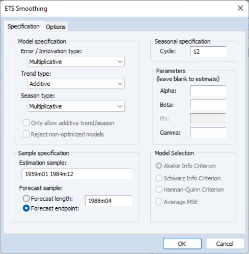
To perform exponential smoothing in EViews, open the series and choose to bring up the dialog:
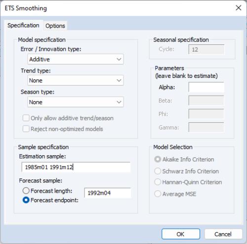
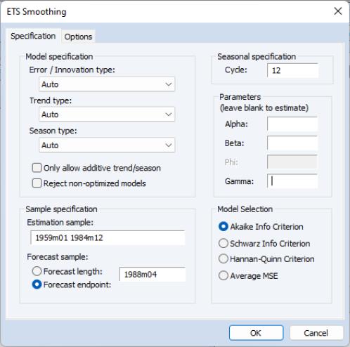
ETS specification
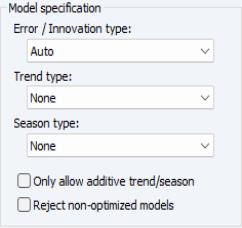
You may use the section of the dialog to specify the type of ETS model you wish to use for smoothing. There is one dropdown menu for each part of the decomposition. By default, EViews employs the additive error, no trend, and no seasonal (A, N, N) model.
In addition to the component choices outlined in
“ETS Decomposition” (N, A, AD,
etc.), EViews offers you an choice so you may specify that the component specification will be chosen using model selection techniques.
For the calculational efficiency, EViews provides two options to reduce the number of available ETS smoothing models. The checkbox lets you choose from models with additive trend and seasonal components only. The checkbox lets you exclude models for which the estimation procedure did not converge from model comparison.
Seasonal specification
If you have specified a seasonal component or elected to select the seasonal specification using model selection, the edit field lets you specify the m length of seasonality. The default cycle setting will depend on the workfile structure (4 for quarterly, 12 for monthly, 2 for all others).
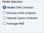
Model selection
When you choose for any of the component types, EViews displays options which let you specify the model selection procedure. You may choose between minimizing one of the information criteria (, , ) or finding the model with the best within sample one-step predictive forecast by minimizing the .
Parameters
The section of the dialog lets you specify fixed values for the smoothing parameters in your model. If you enter a numeric value in one of the edit fields, EViews will fix the parameter at that value and remove it from the set of parameters to be estimated. Leaving a field blank instructs EViews to estimate the parameter.
Note that any user-specified parameter values should fall within the parameter bounds outlined in
Equation (11.95).
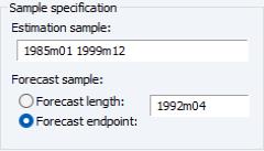
Estimation Sample
The section consists of two settings: the estimation sample, and the forecast end point.
The edit field identifies the contiguous sample that will be used for estimation of the smoothing model. You should enter a single date pair. Note that the ETS procedure does not allow for missing values in the source series.
The lets you specify the end point of your forecast sample. Note that the forecast start point is fixed as the first observation after the estimation sample. For example, if the estimation sample is given as “1985m01 1991m12” and the forecast end point is given as “1992m04”, then EViews will perform exponential smoothing analysis for the estimation sample and forecast the remaining periods (i.e. “1992m01 1992m04”).
Estimation Control
To specify the options for controlling estimation, click on the tab.
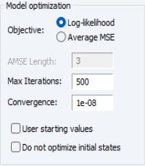
The section allows you to specify the optimization objective function, maximum iterations and convergence, and starting values, and to indicate whether you wish to treat the initial state values as parameters or to use the ad hoc method for computing the initial states.
• : you can choose the objective function which needs to be optimized over, either likelihood based () or forecast error based ().
• : If the average MSE objective function is chosen as the object, the AMSE length
h described in
Equation (11.98) should be specified in the edit field.
• and : Lets you control the iterative process by specifying the maximum number of iterations and convergence criterion.
• By default, starting parameters are set to EViews supplied values, but you may select the checkbox to use the existing values in the C coefficient vector.
• Select the box to use the ad hoc method for computing the initial states.
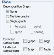
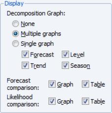
Display
The section provides options for showing the results of the ETS procedure in graph or table form.
The top portion of the section lets you specify the display of the component results in single or multiple graphs. If you select , EViews will display the selected , , , and components in separate graphs. If you select , all of the selected components will be included in a single graph.
If the ETS specification in the page of the dialog (
“ETS specification”) contains any automatically chosen components, EViews will offer you the option of displaying a graph or table of the forecast and likelihood values used to forecast and/or likelihood values used in the model selection procedure. Simply select the appropriate Graph or Table checkbox to include a component. The results will be displayed along with the estimation results.
Output Series
The section of the tab lets you specify the smoothing process output series names. By default EViews will create a new series in the workfile with the final smoothed (and possibly forecasted) series. The name of the created series will be the same as the original series name, with an “_SM” appended to the end. You can change this name using the edit field.
You may elect to save the individual level, trend and seasonal components of the smoothed series output to your workfile by entering a name for those output series in the , , and fields.
Illustration
To illustrate estimation and smoothing using an ETS model, we forecast monthly housing starts (HS) for the period 1985m01–1988m12. These data are provided in the workfile “Hs.WF1”.
We will use the multiplicative error, additive trend, and multiplicative seasonal (M, A, M) model to estimate parameters using data from 1959m01–1984m12 and to smooth and forecast for 1985m1–1988m12.
First, load the workfile, open the HS series, and select ....
Change the drop-down menus to (M, A, M), set the to “1959 1984” or “1959m01 1984m12”, set the t to “1988m04”, and leave the remaining settings at their default values. When you click OK, EViews estimates the ETS model, displays the results, and saves the smoothed results in the HS_SM series in the workfile.
The results are divided into four parts. The first part of the table shows the settings employed in the ETS procedure, including the sample employed for estimation and the estimation status.
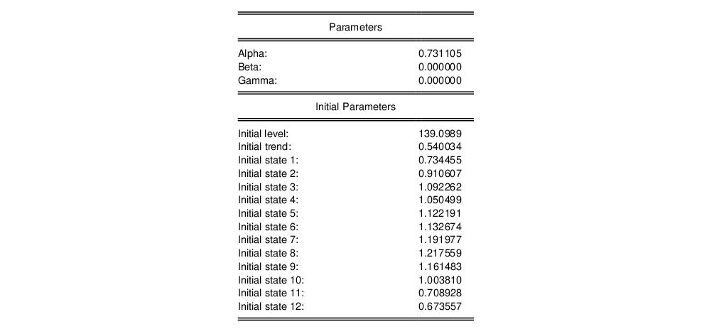
Here we see that we have estimated an (M, A, M) model using data from 1959 to 1984, and that the estimator converged, but with some parameters at boundary values.
The next section of the table shows the smoothing parameters

and initial states

. Note the presence of the boundary zero values for

and

, which indicate that the seasonal and trend components do not change from their initial values.
The bottom portion of the table output contains summary statistics for the estimation procedure:
Most of these statistics are self-explanatory. The reported “Compact Log-likelihood” is simply the log-likelihood value absent inessential constants, and is provided to facilitate comparison with results obtained from other sources.
For comparison purposes, it may be useful to consider the ETS model obtained using model selection. To perform model selection, fill out the dialog as before, but set each of the specification drop-down menus to .
Note that at the default settings, the best model will be selected using the Akaike Information Criterion.
Next, click on the tab and set the options to show the forecast and all of the elements of the decomposition in Multiple graphs, and to produce graphs and tables for the forecast and likelihood comparisons of all of the models considered by the model selection procedure.
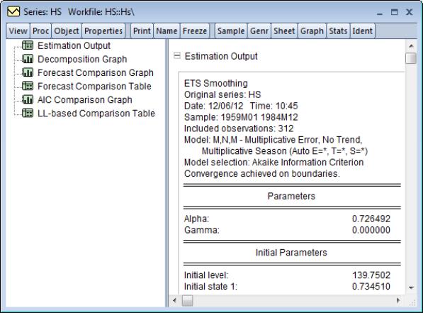
Click on OK to perform the smoothing. Since EViews will be producing several types of output for the procedure, the results will be displayed in a spool:
The left output pane allows you to select the output you wish to display. Simply click on the output you wish to display or use the scroll bar on the right side of the window to move from output to output.
The contains the specification, estimated smoothing and initial parameters, and summary statistics. The top portion of the output,
shows that the Akaike information criterion selected ETS model is an (M, N, M) specification, with level smoothing parameter estimate

, and the seasonal parameter

estimated on the boundary.
The summary statistics indicate that this specification is superior to the earlier (M, A, M) model,
on the basis of all three of the information criteria and the average mean squared error, though the likelihood is lower and the SSR and RMSE are both slightly higher in the selected model.
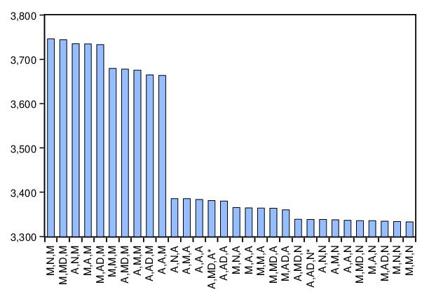
Clicking on the AIC comparison graph in the spool, we see the results for all candidate models:
Note that the selected (M, N, M) and the original (M, A, M) model are among the five specifications with relatively high AIC values.
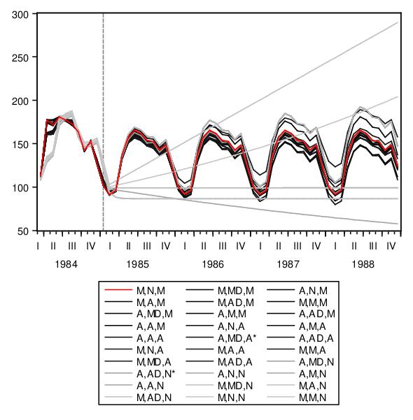
The forecast comparison graph shows the forecasts for the candidate models:
The graph shows both the last few observations of in-sample forecasts and the out-of-sample forecasts for each of the possible ETS specifications.
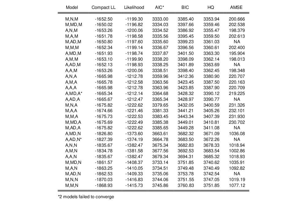
In addition, our chosen ETS display settings produced both the likelihood table which contains the actual likelihood and Akaike values for each specification, and the forecast comparison table, which presents a subset of the values displayed in the graph. For example, the likelihood table consists of
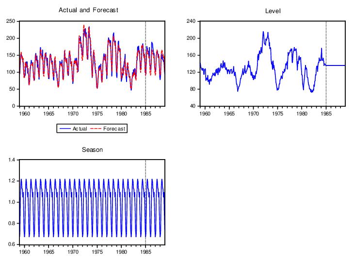
Lastly, the spool contains a multiple graph containing the actual and forecasted values of HS over the estimation and forecast period, along with the decomposition of the series into the level and seasonal components.

 of
of  is computed recursively, by evaluating:
 is the damping (or smoothing) factor. The smaller is the
  , the smoother is the
  series. By repeated substitution, we can rewrite the recursion as
 is a weighted average of the past values of
  , where the weights decline exponentially with time.
 is the end of the estimation sample.
 and a value for
  . EViews uses the mean of the initial
  observations of
  to start the recursion (where
  is the number of observations in the sample). Bowerman and O’Connell (1979) suggest that values of
  around 0.01 to 0.30 work quite well. You can also let EViews estimate
  to minimize the sum of squares of one-step forecast errors.
 is defined by the recursions:
 is the single smoothed series and
  is the double smoothed series. Note that double smoothing is a single parameter smoothing method with damping factor
  .
. 
 and slope
  .
.  is given by,


 are the damping factors and
  is the seasonal frequency specified in the Cycle for Seasonal field box.
 estimates.
 is given by:
 and
and  are the permanent component and trend as defined above in
Equation (11.60) and
  are the additive seasonal factors. The three coefficients are defined by the following recursions:
 are the damping factors and
  is the seasonal frequency specified in the Cycle for Seasonal field box.
 estimates.
  is given by:

 are the damping factors. This is an exponential smoothing method with two parameters.
 and slope
  .
.  . The condition
  only restricts the seasonal factors from changing over time so there are still (fixed) nonzero seasonal factors in the forecasts.
 , and trend
  at the end of the estimation sample that are used for post-sample smoothed forecasts.
 used in the forecasts are also displayed. The smoothed series in the workfile contains data from the beginning of the estimation sample to the end of the workfile range; all values after the estimation period are forecasts.
 may be decomposed into three components, trend (T), seasonal (S), and error (E), where the trend term characterizes the long-term movement of
  , the seasonal term corresponds to a pattern with known periodicity, and the error term is the irregular, unpredictable component of the series.
 . We may have a purely additive model, say
  or
or  , a pure multiplicative model like
  or
or  , or models which mix the two, as in
  or
or 

 possible ETS models associated with these choices.
 may itself be decomposed into a level term (
 ) and a growth term (
 ) in several ways. Following Hyndman, et al. (2008) we let
  be the trend forecast
  periods out, and let
  be a damping parameter. The five different trend types corresponding to different assumptions about the growth term are given by:


 .
. ) which is always present, and a growth term (
 ) which may or may be present, depending on the trend specification. If we let
  represent included seasonal terms, we may define the general following
  -dimensional state vector:

 and
and  are known continuous scalar functions,
  and
and  are known continuously functions with continuous derivatives from
  and
and  where
where  independent of past realizations of
  and
and  .
. equation represents how the various state variable components
  are combined to express the series in terms of a smoothed forecast
  and the prediction error
  . The multiple functions are a notational device for writing the additive and multiplicative errors in compact form. With additive errors we have
  so that
 , yielding
 equations outline the process by which the component estimates are updated using the previous period’s estimates and the current prediction error
  . For the ETS models considered here, we may think of the updating smoothing equations as being weighted averages of a term which depends on the current prediction error (and prior states), and one which depends on the prior states. The resulting state equations are extended versions of those outlined by Hyndman, et al. (2002), and take the general form:
 ,
,  and
and  are functions of the prediction error and lagged states, and
  is a function of the lagged states.
  is the damping parameter for linear trend models and
  is the damping parameter for multiplicative trend models. In the absence of a damping, the parameters are set to 1.
 . For this linear error specification, obtain the prediction error equation


 , and functions
  ,
,  , and
, and  .
. and let
  be the one-period ahead forecast of
  since we have an additive trend specification with no seasonal component.

 and
and  .
. 
 and
and  .
.
 ). Define the state vector
  . The one-period ahead forecast is


 and let
  be the one-period ahead forecast of
  . Then the prediction error decomposition is


 (since we have a multiplicative damped trend) and
  .
.

 , and values for the initial states
  , we may use the ETS state and prediction equations to obtain smoothed estimates of the unobserved components and the underlying series. Typically the parameters are estimated. The initial states are either estimated or assigned ad hoc values.
 , nor the initial seasonal states
  . We will use
  and
and  to refer to the relevant subsets for a given model which are to be estimated.
 . The traditional approach has assigned the following restrictions on the parameters to ensure model stability:
 . For seasonal data, compute a linear trend using linear regression on the first ten seasonally adjusted values against a time series. And then set the initial level
  to be the intercept of the trend.
 to be the slope of the trend. For multiplicative trends, set
  where
where  and
and  denote the intercept and slope of the fitted trend, respectively.
 moving average through the first few years of data. Denote this set of values
  . For additive seasonality, detrend the data to obtain
  . For multiplicative seasonality, detrend the data to obtain
  . Compute initial seasonal indices
  by averaging the detrended data for each season. Normalize these seasonal indices so that they add to zero for additive seasonality, and add to
  for multiplicative seasonality.
 and, optionally, the initial states
  .
.
 ,
,  , and
, and  using the Broyden, Fletcher, Goldfarb and Shanno (BFGS) algorithm.
 -step forecasts of the specified ETS model.
 . The
. The  -step ahead forecast error is defined as
 are obtained by recursively solving the state equations assuming
  in each period.
 -step forecasts is defined as
 and
and  using BFGS.
 we have
 , and
, and
 . Then the
  -step ahead forecasts are


 are the maximized values and p is the number of parameters in
  plus the number of the estimated initial states in
  . The model that minimizes the AIC (BIC, or HQ) across all available models is adopted.
 and using the prediction errors to update the state estimates.




 and initial states
  . Note the presence of the boundary zero values for
  and
and  , which indicate that the seasonal and trend components do not change from their initial values.


 , and the seasonal parameter
  estimated on the boundary.
