Forecast Averaging
Economic forecasters often have a variety of different models and forecasts of the same variable from which to choose. These models and forecasts may differ in the underlying assumptions, or may employ different information. Traditionally the forecasting decision was to pick which single forecast was “best” out of the individual forecasts available.
However, a number of studies have shown that averaging forecasts is more accurate than choosing a single best forecast. Timmermann (2006) offers a good overview of such studies, citing Clemen (1989) and Makridakis and Hibon (2000) in particular.
Forecast averaging, or forecast combining, is a methodology for combining multiple forecasts into a single forecast. The methods and ideas behind forecast averaging are founded in forecast evaluation and model selection techniques. Rather than calculating a measure of how good each forecast is, and then selecting the best forecast, the forecast evaluation measures are used to produce weights for calculating a weighted average of all the forecasts.
Methodology
Forecast averaging methods typically employ a simple weighted average computation—at each observation of the forecast sample, the cross-forecast average is computed, with different forecasts assigned different weights.
It is possible to compute complicated weighting schemes that allow the weights to vary through the forecast period. EViews, however, offers methods that generally employ constant weights through time: simple mean, least squares, mean square error, mean square error ranks, smoothed AIC, approximate Bayesian model averaging. Notable exceptions where weights are time-varying are the trimmed mean and simple median methods).
We will briefly discuss each method in turn.
Simple Mean
The simple mean averaging method takes the arithmetic mean of the forecasts at each observation in the forecast sample. Note that in the simple mean method, every forecast is given the same weight.
Trimmed Mean
The trimmed mean is calculated in the same way as the simple mean, but at each observation the highest

% and the lowest

% of the forecast values are dropped from the mean calculation. Note that the selection of which forecasts to remove as part of the trimming is recalculated at each observation in the forecast sample so that the weights are time-varying—each forecast method may appear in the averaging calculation for some observations but not at others.
Simple Median
The simple median method calculates the median of the forecasts at every observation in the forecast sample. The implicit (0, 1) weights are time-varying as each forecast method may be the median for some observations but not others.
Least Squares Weights
Least squares weighting requires knowledge of the true values of the forecasted variable for some of the forecast period. It is calculated by regressing the forecasts against the actual values and then using the coefficients from the regression as weights. Details of this method are outlined in the Handbook of Economic Forecasting, Vol 1, page 159. EViews calculates the most general model which includes an intercept to the regression.
This method does not require that the underlying individual forecasts are unbiased, and the resulting average can lie outside the range of the underlying forecasts.
Mean Square Error (MSE) Weights
MSE weighting, proposed by Stock-Watson (2001), compares the individual forecasts with the actual values over some forecast period. The MSE of each forecast is computed and used to form individual forecast weights:
 | (11.51) |

is used to raise the MSE to different powers.

is the most commonly used power, and yields a weight based on the ratio of each forecast’s MSE to the total of all the MSEs.
MSE Ranks
Aiolfi and Timmermann’s (2006) MSE ranks method is similar to the MSE Weights method outlined above, but rather than computing the ratio of MSE vales, this method computes the MSE of each forecast, ranks them, and then computes the ratio of the inverse of the ranks. so that each forecast’s weight is its rank divided by the sum of all ranks.
Smoothed AIC Weights
Smoothed AIC weights use the Akaike information criterion from the original estimation/model that produced each forecast, then calculates the weights as:
 | (11.52) |
Smoothed AIC weights can only be computed if EViews has access to the underlying estimation results with associated AIC values.
Approximate Bayesian Model Averaging Weights
EViews calculates BMA weights in a similar fashion to Smoothed AIC weights, but uses the Schwarz criterion instead of the AIC:
 | (11.53) |
The approximate BMA uses the BIC to give a large sample approximation to computing Bayes factors. In finite samples the BIC may overly weight parsimonious models.
Forecast Averaging in EViews
To perform forecast averaging in EViews, you must start with a series representing the data to be forecasted. Some of the forecast weighting techniques require actual data to calculate the weights, and in these cases this series should contain actual values for the variable being forecasted for at least some of the observations for which forecast values are available.
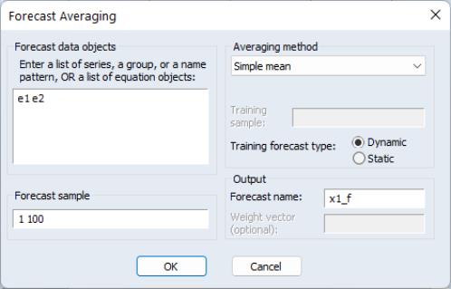
To begin, open up the series and click on , which will open the Forecast Averaging dialog box:
The Forecast data objects box specifies the forecasts to be used for averaging. Forecasts can be entered either as a collection of series (in which case the names of the series, a series naming pattern, or the name of a group are entered), or as a list of equation objects. If equation objects are entered, EViews will automatically perform a dynamic forecast over the forecast period from each of those equation objects to generate the forecast data.
When using equation objects, rather than forecast series, as the forecast data, the following should be noted:
• Each equation must have an identical dependent variable, which is identical to the series from which you are performing the forecast evaluation. i.e., if you are forecasting from series Y, each equation must have Y as the dependent variable. Currently transformations (such as LOG(Y)) are not allowed.
• If using smoothed AIC or BMA/SIC averaging methods, the weight calculations are only strictly valid if the underlying estimation objects were estimated on identical samples. It is up to the user to ensure that the samples are identical.
• Only equation objects are allowed. If a different type of estimation object (system, VAR, Sspace, etc.) is used, or if forecast was obtained from a non-EViews estimation source, the forecasts cannot be specified by equation.
• If using one of the MSE based or the OLS based weighting methods, historical forecasts (along with actual values) are needed for use in the weighting calculation. Note that EViews will not re-estimate the equations, it will use the same coefficient values for both the historical forecast and the actual forecasts, based on whatever sample was used when the equation were originally estimated. If you wish to use different estimation samples for the comparison forecast and actual forecast, you must perform the estimation and forecasts manually and specify the forecast data by series.
The Forecast sample box specifies the sample over which the forecasts will be averaged.
The Averaging method area specifies the forecast averaging procedure. The first dropdown selects the specific method of averaging. If the Trimmed mean averaging method is selected, the Percent: box specifies the level of trimming (from both ends). If the Mean square error method is selected, the Power: box specifies the power to which the MSE is raised.
Note the Smooth AIC weights and SIC weights selections are only available if a list of equations is entered in the Forecast data objects box, since they require information from the estimation rather than just the raw forecast data.
The Least-squares, Mean square error, MSE ranks, Smooth AIC weights, and SIC weights averaging methods require a training sample - a sample over which the averaging weights are computed. If any of these averaging methods are selected, a sample must be entered in the Training sample: box. If a list of equations is entered in the Forecast data objects box, the Training forecast type: radio buttons select which type of forecast is used over the training sample.
The Output section allows specification of the name of the final averaged forecast series (by default given a name equal to the underlying series plus “_f”. If the selected averaging method requires calculation of averaging weights, the weighting vector can be saved into the workfile by entering a name in the Weight vector (optional): box.
An Example
As an example of forecast averaging in EViews, we average six monthly forecasts of electricity demand in England and Wales, using the workfile elecdmd.wf1. This workfile contains monthly electricity demand data from April 2005 until April 2014 (in the series ELECDMD), along with five evaluation sample forecasts of electricity demand (series ELECF_FE1-5), and five out-of-sample forecasts (series ELECF_FF1-5). The different forecast series correspond to different five different models used to generate forecasts.
Each of the out-of-sample forecast series contains actual data until April 2013, and then forecast data from May 2013 until December 2015. There is a year of overlap (May 2013 until April 2014) where actual data exists during the forecast period.
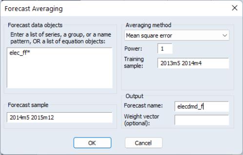
We will use forecast averaging to create a combination forecast from our five individual forecast series. To begin, we open the ELECDMD series and click on and enter the names of our forecast series in the Forecast data objects box of the Forecast Averaging dialog, using the naming patter ELEC_FF* (to indicate any series matching that pattern):
We set the forecast sample to “2014m5 2015m12”. We select as the average method, with data between 2013M5 and 2014M4 used to calculate the MSE. We save the final averaged series in a new series called ELECDMD_F.
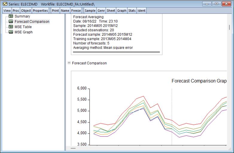
The output of the procedure is as follows:
The top of the output provides summary information about the averaging procedure, including the time and date it was performed, the number of observations included (20 in this case) and the number of forecasts used in the averaging calculation, as well as the method used.
EViews also produces a graph of each of the individual forecasts, and the calculated average, allowing a quick visual comparison.
 % and the lowest
  % of the forecast values are dropped from the mean calculation. Note that the selection of which forecasts to remove as part of the trimming is recalculated at each observation in the forecast sample so that the weights are time-varying—each forecast method may appear in the averaging calculation for some observations but not at others.
 % and the lowest
  % of the forecast values are dropped from the mean calculation. Note that the selection of which forecasts to remove as part of the trimming is recalculated at each observation in the forecast sample so that the weights are time-varying—each forecast method may appear in the averaging calculation for some observations but not at others.
 is used to raise the MSE to different powers.
  is the most commonly used power, and yields a weight based on the ratio of each forecast’s MSE to the total of all the MSEs.


