Forecast Evaluation
When constructing a forecast of future values of a variable, economic decision makers often have access to different forecasts; perhaps from different models they have created themselves or from forecasts obtained from external sources. When faced with competing forecasts of a single variable, it can be difficult to decide which single or composite forecast is “best”. Fortunately, EViews provides tools for evaluating the quality of a forecast which can help you determine which single forecast to use, or whether constructing a composite forecast by averaging would be more appropriate.
Methodology
Evaluation of the quality of a forecast requires comparing the forecast values to actual values of the target value over a forecast period. A standard procedure is to set aside some history of your actual data for use as a comparison sample in which you will compare of the true and forecasted values.
EViews allows you to use the comparison sample to: (1) construct a forecast evaluation statistic to provide a measure of forecast accuracy, and (2) perform Combination testing to determine whether a composite average of forecasts outperforms single forecasts.
Forecast Evaluation Statistics
EViews offers four different measures of forecast accuracy; RMSE (Root Mean Squared Error), MAE (Mean Absolute Error), MAPE (Mean Absolute Percentage Error), and the Theil Inequality Coefficient. These statistics all provide a measure of the distance of the true from the forecasted values.
Suppose the forecast sample is
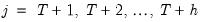
, and denote the actual and forecasted value in period

as

and

, respectively. The forecast evaluation measures are defined as:
Root Mean Squared Error | |
Mean Absolute Error | |
Mean Absolute Percentage Error | |
Theil Inequality Coefficient | |
Combination Tests
To test whether an average, or combination, of the individual forecasts may perform better than the individual forecasts themselves, EViews offers the Combination Test, or Forecast Encompassing Test of Chong and Hendry (1986) and refined by Timmermann (2006). The idea underlying this test is that if a single forecast contains all information contained in the other individual forecasts, that forecast will be just as good as a combination of all of the forecasts. A test of this hypothesis can be conducted by performing a regression of the model:
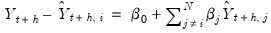 | (11.19) |
where

is the vector of actual values over the forecast period and

is the vector of forecast values over the same period for forecast
i. A test for whether forecast
i contains all the information of the other forecasts may be performed by testing whether
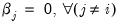
; if the difference between the true values and the forecasted values from forecast
i is not related to the forecasts from all other models, then forecast
i can be used individually. If the differences are affected by the other forecasts, then the latter forecasts should be included in the formation of a composite forecast.
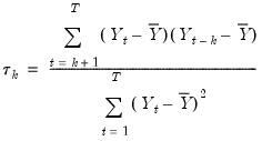
Diebold-Mariano Test
The Diebold-Mariano test is a test of whether two competing forecasts have equal predictive accuracy. For one-step ahead forecasts, the test statistic is computed as:
 | (11.20) |
where
 | (11.21) |
and

,

is either a squared or absolute difference between the forecast and the actual,
 | (11.22) |
or
 | (11.23) |
where

and

are the mean and sample standard deviation of

. (Note that while Diebold and Mariano define an

-step statistic, EViews only computes the one-step version.)
Following Harvey, Leybourne, and Newbold (HLN), EViews calculates the standard deviation using a small-sample bias corrected variance calculation.
The test-statistic follows a Student’s
t-distribution with

degrees of freedom.
EViews will only display the Diebold-Mariano test statistic if exactly two forecasts are being evaluated.
Forecast Evaluation in EViews
To perform forecast evaluation in EViews, you must have a series containing the observed values of the variable for which you wish to evaluate forecasts. To begin, open up the series and click on , which will open the Forecast Evaluation dialog box:
The Forecast data objects box specifies the forecasts to be used for evaluation. Forecasts can be entered either as a collection of series (in which case the names of the series, a series naming pattern, or the name of a group are entered), or as a list of equation objects. If equation objects are entered, EViews will automatically perform a dynamic forecast over the forecast period from each of those equation objects to generate the forecast data.
When using equation objects, rather than forecast series, as the forecast data, the following should be noted:
• Each equation must have an identical dependent variable, which is identical to the series from which you are performing the forecast evaluation. i.e., if you are forecasting from series Y, each equation must have Y as the dependent variable. Currently transformations (such as LOG(Y)) are not allowed.
• If using smoothed AIC or BMA/SIC averaging methods, the weight calculations are only strictly valid if the underlying estimation objects were estimated on identical samples. It is up to the user to ensure that the samples are identical.
• Only equation objects are allowed. If a different type of estimation object (system, VAR, Sspace, etc.) is used, or if forecast was obtained from a non-EViews estimation source, the forecasts cannot be specified by equation.
• If using one of the MSE based or the OLS based weighting methods, historical forecasts (along with actual values) are needed for use in the weighting calculation. Note that EViews will not re-estimate the equations, it will use the same coefficient values for both the historical forecast and the actual forecasts, based on whatever sample was used when the equation were originally estimated. If you wish to use different estimation samples for the comparison forecast and actual forecast, you must perform the estimation and forecasts manually and specify the forecast data by series.
The Evaluation sample box specifies the sample over which the forecasts will be evaluated.
The Averaging methods (optional) area selects which forecast averaging methods to evaluate. For more details on each averaging method, see FORECAST AVERAGING ENTRY. If the Trimmed mean averaging method is selected, the Percent: box specifies the level of trimming (from both ends). If the Mean square error method is selected, the Power: box specifies the power to which the MSE is raised.
Note the Smooth AIC weights and SIC weights options are only available if a list of equations is entered in the Forecast data objects box, since they require information from the estimation rather than just the raw forecast data.
The Least-squares, Mean square error, MSE ranks, Smooth AIC weights, and SIC weights averaging methods require a training sample - a sample over which the averaging weights are computed. If any of these averaging methods are selected, a sample must be entered in the Training sample box. If a list of equations is entered in the Forecast data objects box, the Training forecast type radio buttons select which type of forecast is used over the training sample.
An Example
As an example of forecast evaluation in EViews, we evaluate six monthly forecasts of electricity demand in England and Wales, using the workfile “elecdmd.wf1”. This workfile contains monthly electricity demand data from April 2005 until April 2014 (in the series ELECDMD), along with five evaluation sample forecasts of electricity demand (series ELECF_FE1–ELECF_FE5), and five out-of-sample forecasts (series ELECF_FF1–ELECF_FF5). The different forecast series correspond to different five different models used to generate forecasts.
Each of the evaluation sample forecast series contains actual data until December 2011, and then forecast data from January 2012 until December 2013.
We will evaluate the five models’ forecast accuracy using the evaluation sample forecast series. To begin, we open the ELECDMD series and click on and enter the names of our forecast series in the Forecast data objects box of the Forecast Evaluation dialog:
We set the evaluation sample to “2013M1 2013M12”, giving us twelve months of forecasts to evaluate. We choose to evaluate each of the available averaging methods, and set the training sample for the , and methods to be “2012M1 2012M12”.
The top of the output provides summary information about the evaluation performed, including the time and date it was performed, the number of observations included (12 in this case) and the number of forecasts evaluated, including the averaging methods.
The “Combination tests” section displays the results of the combination test for each of the individual forecasts. In our case the null hypothesis is non-rejected for each of the forecasts, other than the first, which is rejected at a 5% level.
The “Evaluation statistics” section shows the RMSE, MAE, MAPE and Theil statistics for each of the five forecasts, along with the five averaging methods. The trimmed mean averaging method could not be calculated with only 5 forecast series.
EViews has shaded the forecast or averaging method that performed the best under each of the evaluation statistics. In our case the MSE ranks method outperforms every other forecast or averaging method in each of the evaluation criteria.
EViews also produces a graph of each of the individual forecasts, the averages, and the actual values over the training and evaluation periods, allowing a quick visual comparison of each: