Generate by Classification
The series classification procedure generates a categorical series using ranges, or bins, of values in the numeric source series. You may assign individuals into one of

classes based any of the following: equally sized ranges, ranges defined by quantile values, arbitrarily defined ranges. A variety of options allow you to control the exact definition of the bins, the method of encoding, and the assignment of value maps to the new categorical series.
We illustrate these features using data on the 2005 Academic Performance Index (API) for California public schools and local educational agencies (“Api05btx.WF1”). The API is a numeric index ranging from 200 to 1000 formed by taking the weighted average of the student results from annual statewide testing at grades two through eleven.
The series API5B contains the base API index. Open the series and select to display the dialog. For the moment, we will focus on the and the sections.
Output
In the section you will list the name of the target series to hold the classifications, and optionally, the name of a valmap object to hold information about the mapping. Here, we will save the step size classification into the series API5B_CT and save the mapping description in API5B_MP. If the classification series already exists, it will be overwritten; if an object with the map name already exists, the map will be saved in the next available name (“API5B_MP01”, etc.).
Specification
The section is where you will define the basic method of classification. The dropdown allows you to choose from the four methods of defining ranges: , , , . The first two methods specify equal sized bins, the latter two define variable sized bins.
Step Size
We will begin by selecting the default method and entering “100” and “200” for the and edit fields. The step size method defines a grid of bins of fixed size (the step size) beginning at the specified grid start, and continuing through the grid end. In this example, we have specified a step size of 100, and a value of 200. The is left blank so EViews uses the data maximum extended by 5%, ensuring that the rightmost bin extends beyond the data values. These settings define a set of ranges of the form: [100, 200), [200, 300), ..., [1000, 1100). Note that by default the ranges are closed on the left so that we say
lies in the first bin if

.
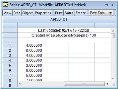
Click on to accept these settings, then display the spreadsheet view of API5B_CT. We see that observations 1 and 3 fall in the [500, 600) bin, while observations 4 and 5 fall in the [400, 600) bin. Observations 2 and 6 were NAs in the original data and those values have been carried over to the classification.
Keep in mind that since we have created both the classification series and a value map, the values displayed in the spreadsheet are mapped values, not the underlying data. To see the underlying classification data, you may go to the series toolbar and change the setting to .
Opening the valmap API5B_MP, we see that the actual data in API5B_CT are integer values from 1 to 9, and that observations 1 and 3 are coded as 4s, while observations 4 and 5 are coded as 3s.
Number of Bins
The second method of creating equal sized bins is to select in the dropdown. The label for the second edit field will change from “Bin size” to “# of bins”, prompting you for an integer value
. EViews will define a set of bins by dividing the grid range into
equal sized bins. For example, specifying 9 bins beginning at 200 and ending at 1100 generates a classification that is the same as the one specified using the step size of 100.
Quantile Values
One commonly employed method of classifying observations is to divide the data into quantiles. In the previous example, each school was assigned a value 1 to 9 depending on which of 9 equally sized bins contained its API. We may instead wish to assign each school an index for its decile. In this way we can determine whether a given school falls in the lowest 10% of schools, second lowest 10%, etc.
To create a decile classification, display the dialog, select from the dropdown, and enter the number of quantile values, in this case “10”.
We see that the first 4 (non-NA) values are all in the first decile (<583.8), while observations 7 and 8 lie in the eighth decile [780, 815). As before, these values are the mapped values; the underlying values are encoded with integer values from 1 to 10.
It is worth emphasizing that the mapped values are text representations of the quantile values, akin to labels, and will generally not be displayed in full precision.
Limit Values
You may also define your bins by providing an arbitrary set of two or more limit points. Simply select from the dropdown and provide a list of numeric values, scalars, or vectors. EViews will sort the numbers and define a set of bins using those limits.
Options
EViews provides various options that allow you to fine tune the classification method or to alter the encoding of classification values.
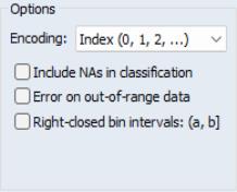
Encoding
The dropdown menu labeled allows you to select different methods of assigning values to the classified observations. By default, EViews classifies observations using the integers 1, 2, etc. so that the observations falling in the first bin are assigned the value 1, observations in the second bin are assigned 2, and so forth.
In addition to the default method, you may elect to use the , the , or the . Each of these encoding methods should be self-explanatory. Note that index encoding is the only method available for classification by quantile values.
Value maps are not created for classifications employing non-index encoding.
NA classification
By default, observations in the original series which are NA are given the value NA in the classification series. If you treat the NA as a category by checking , EViews will assign NAs the index value of 0 in the classification, and will map this value to the label “NA”.
For example, re-running our first example (step size of 100, a grid start value of 200) but keeping NAs, we have the following raw data. Note that the mapped values will be identical to those from the earlier example, so we have switched the series to to see the values for NA:
We see that the observations 2 and 6, which were missing values in the original data, are encoded with the index value 0.
Out-of-Range Values
You may instruct EViews to generate an error if it encounters an observation that does not fall into one of the specified bins; by default, observations that lie outside the bin range are simply assigned an NA.
This option is irrelevant for quantile value classification.
Right-closed Bins
Bins are left-closed by default, so that

lies in the bin defined by

and

if

. To change the non-strict inequality from the left to the right

, you must instruct EViews to use right-closed bins by checking the box . This setting should have little effect, if any, if your data are reasonably continuous.
A Couple of Warnings
In determining whether an observation is in a particular interval, EViews performs comparisons of real numbers to assess, for example, whether

and whether

. We urge you to exercise caution in cases where

and

are finite precision representations of real numbers.
To take a specific example, suppose that we wish to divide the interval from 0 to 1 into bins of size 0.1 (so that our limit points are 0.1, 0.2, 0.3, etc.). Since 0.1 cannot be represented in floating point by a computer, comparisons will be made with numbers that are close to, but not exactly equal to 0.1. As a result, when there are data values approximately equal to the limit points, classifications may behave unexpectedly since they are based on a comparison of two floating point numbers.
A related issue occurs when you classify by number of bins, and set the start or end values equal to the data minimum or maximum. In this situation, depending upon whether you have selected left or right-closed intervals, observations with values equal to the start or end may fall out-of-range.
To illustrate this issue, we extend our example by assuming that we wish to divide the 0–1 range into right-closed bins. Each bin will be of the form [0.1

, 0.1

). with the first interval given by (0, 1]. Now consider classifying those data values that are exactly equal to 0, and note that these values are out-of-range since they lie outside the first interval. The same is true for observations equal to 1 if we have defined left-closed bins. The comparison is more complex if the relevant endpoint is real valued since the out-of-range status would depend upon a floating point comparison.
The obvious recommendation in this latter case are that: (1) you specify at most only one of range start and range end at the data extremes, and (2) if you set either the start or end to the corresponding data extreme, you define the intervals so that they are closed on that end (i.e., starts that equal the minimum have left-closed intervals, and ends that equal the maximum have right-closed intervals) and you set the range so that it extends past the other extreme. Our first example above adopts this strategy, setting the low value to the data minimum (200), setting the step size, and leaving the upper limit unspecified.
More generally, we urge you to exercise caution when defining intervals with real-valued limits.